Fit a Gaussian process to spatial proteomics data

The fitGP function is a helper function to fit GPs with squared exponential co-variances, maximum marginal likelihood

The fitGPmaternPC function is a helper function to fit matern GPs to data with penalised complexity priors on the hyperparameters.

The fitGPmatern function fits matern GPs to data.

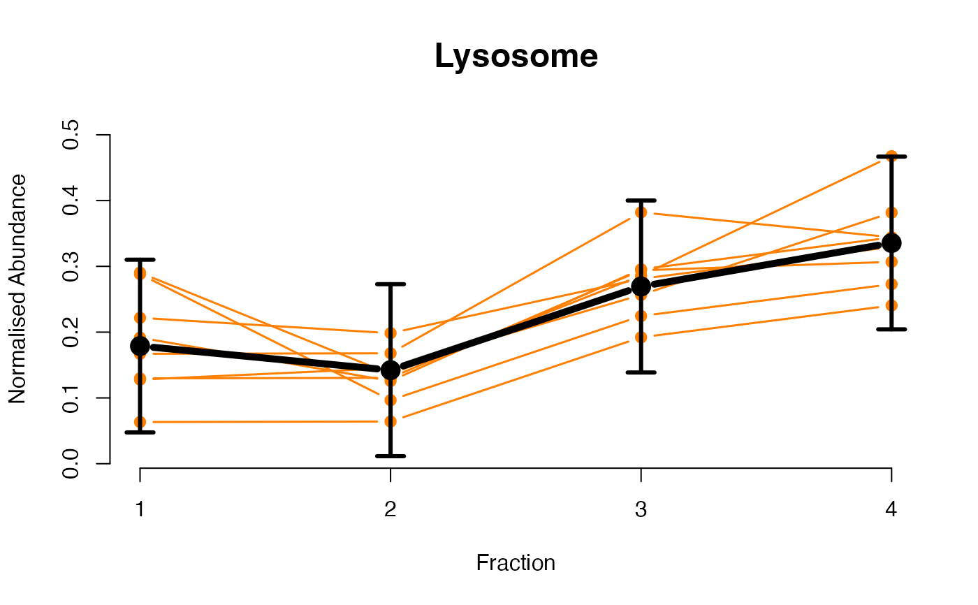
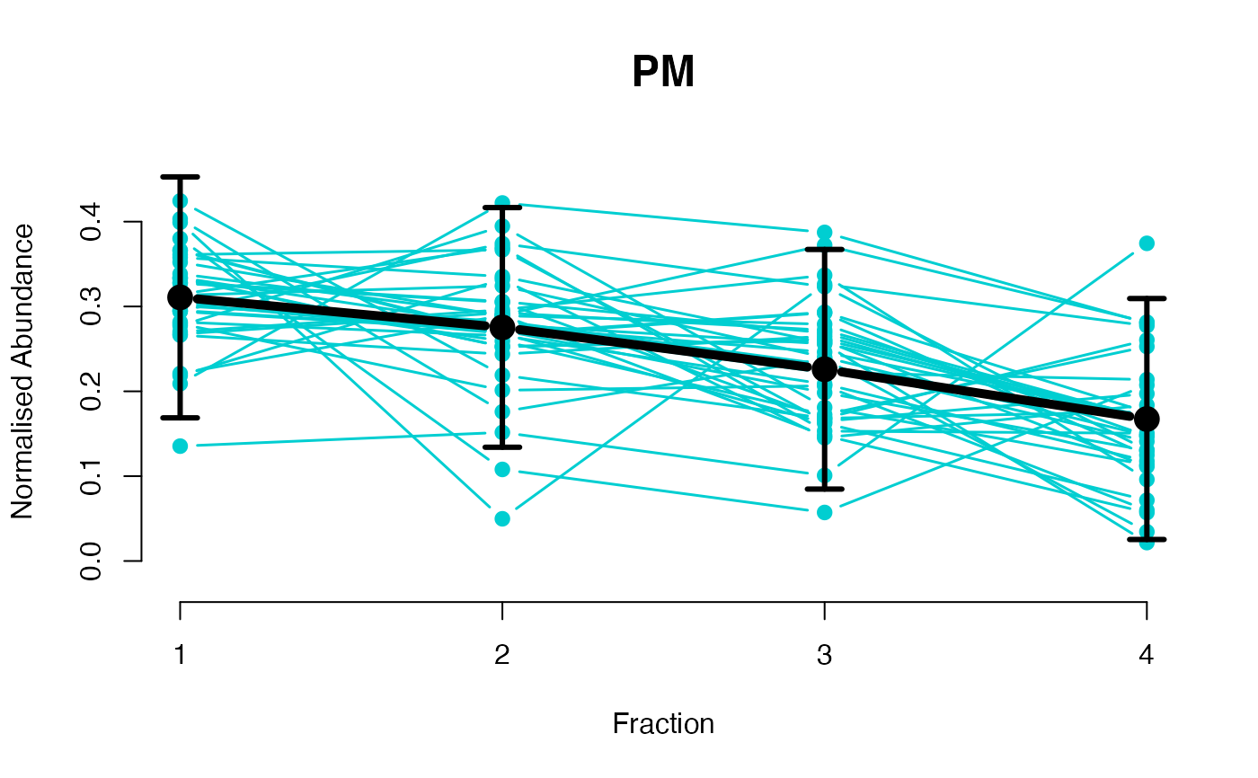
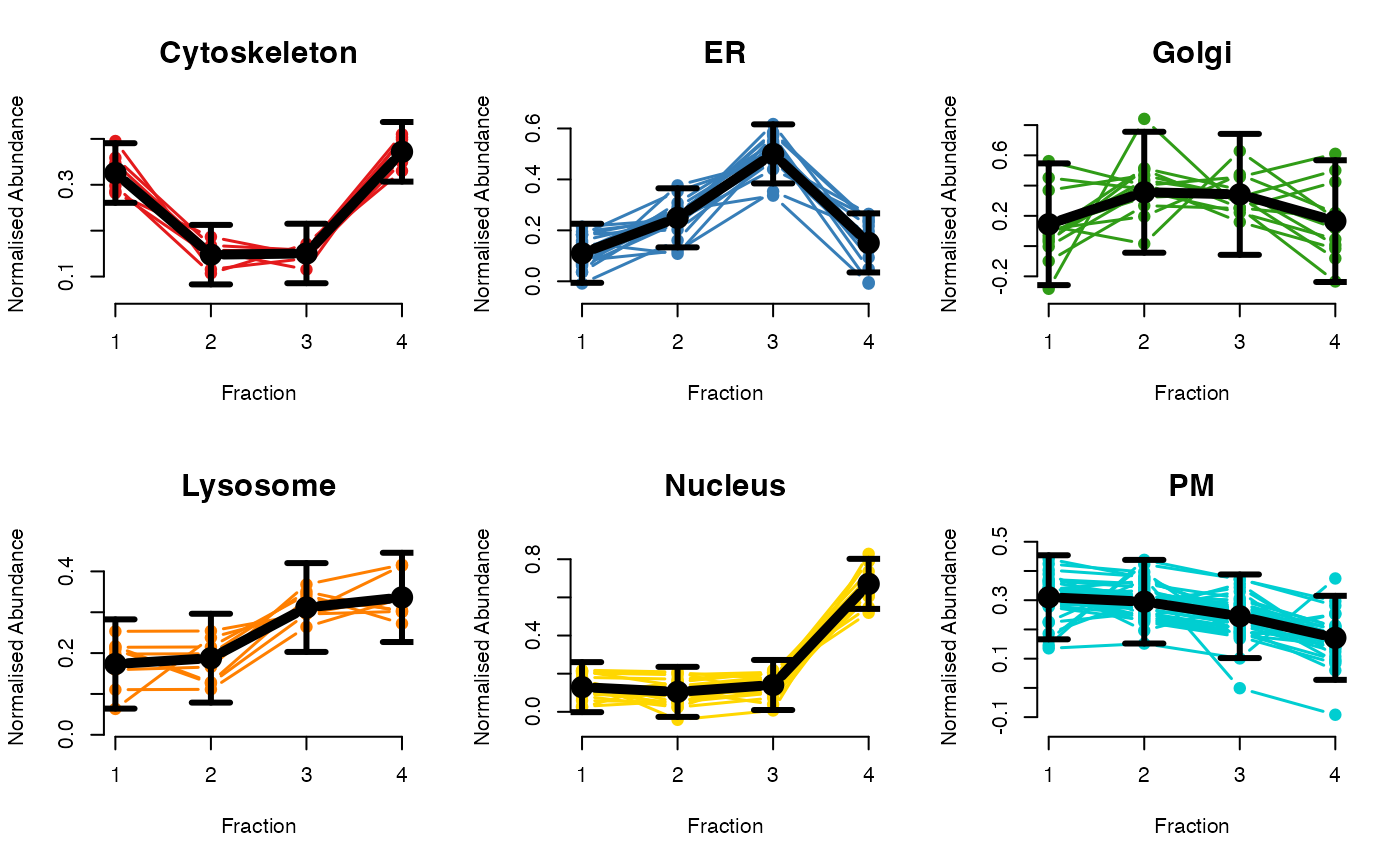
The plotGPmatern function plots matern GPs

fitGP(object = object, fcol = "markers")

fitGPmaternPC(
  object = object,
  fcol = "markers",
  materncov = TRUE,
  nu = 2,
  hyppar = matrix(c(10, 60, 250), nrow = 1)
)

fitGPmatern(object = object, fcol = "markers", materncov = TRUE, nu = 2)

plotGPmatern(object = object, params = params, fcol = "markers")

Arguments

object: A instance of class MSnSet
fcol: feature column to indicate markers. Default is "markers".
materncov: logical indicating whether matern covariance is used.
nu: matern smoothness parameter. Default is 2.
hyppar: The vector of penalised complexity hyperparameters, you must provide a matrix with 3 columns and 1 row. The order is hyperparameters on length-scale, amplitude, variance.
params: The output of running fitGPmatern, fitGPmaternPC or fitGP which is of class gpParams

Value

Returns an object of class gpParams which stores the posterior predictive means, standard deviations, variances and also the MAP hyperparamters for the GP.

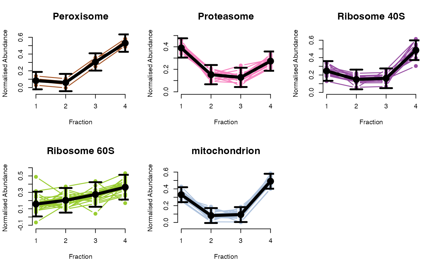
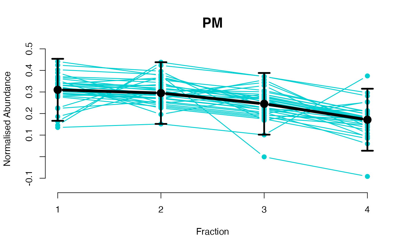
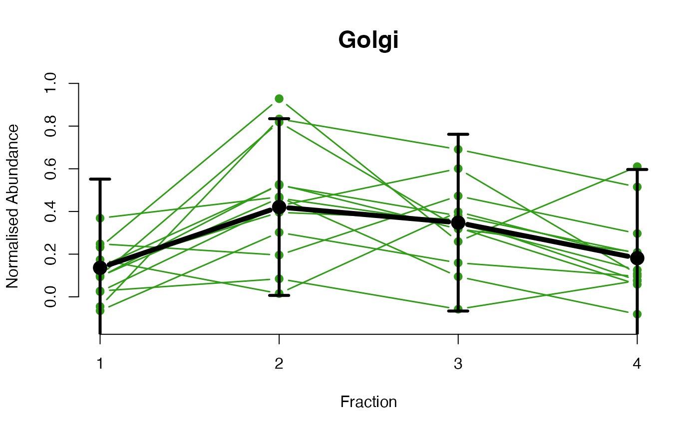
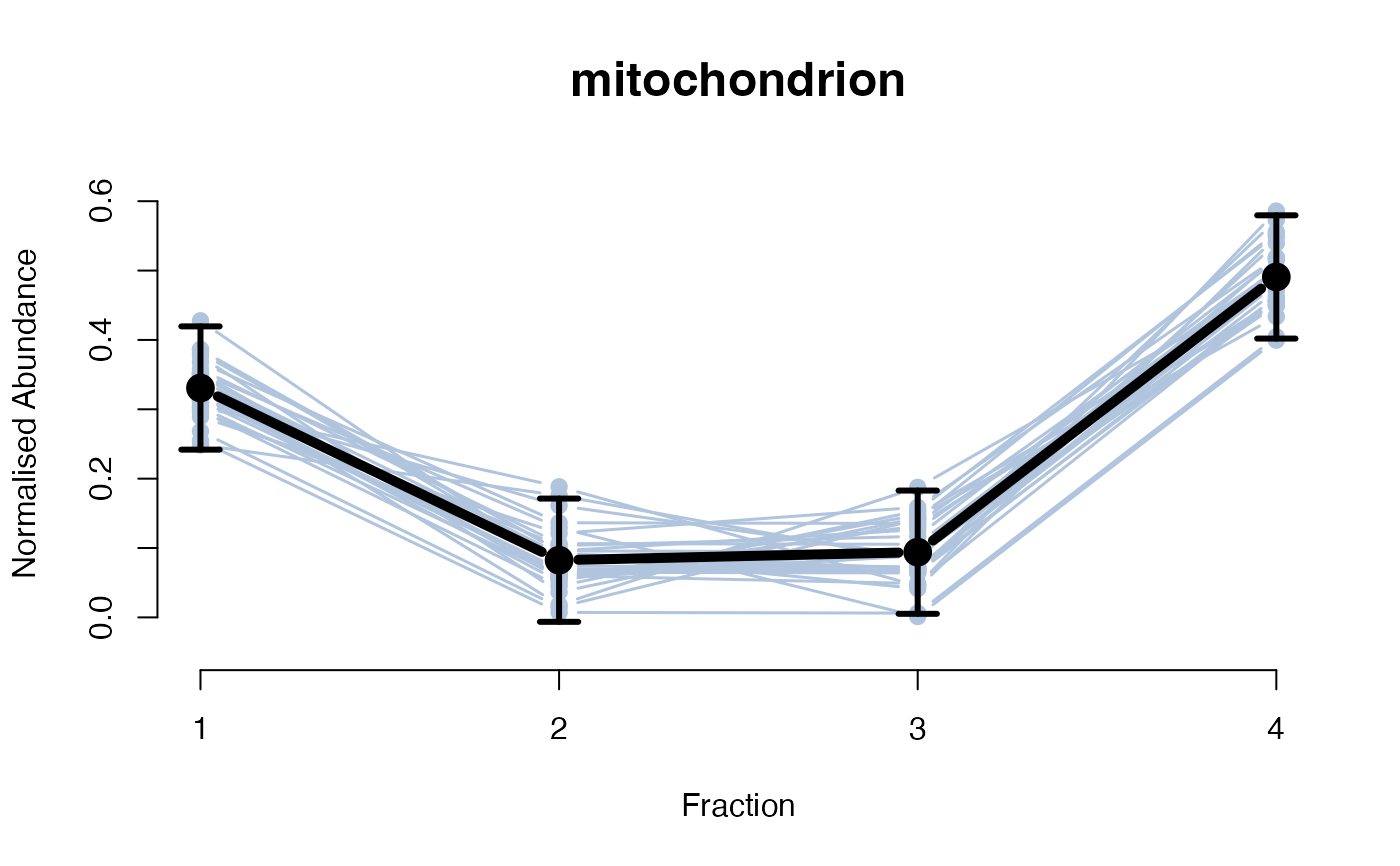
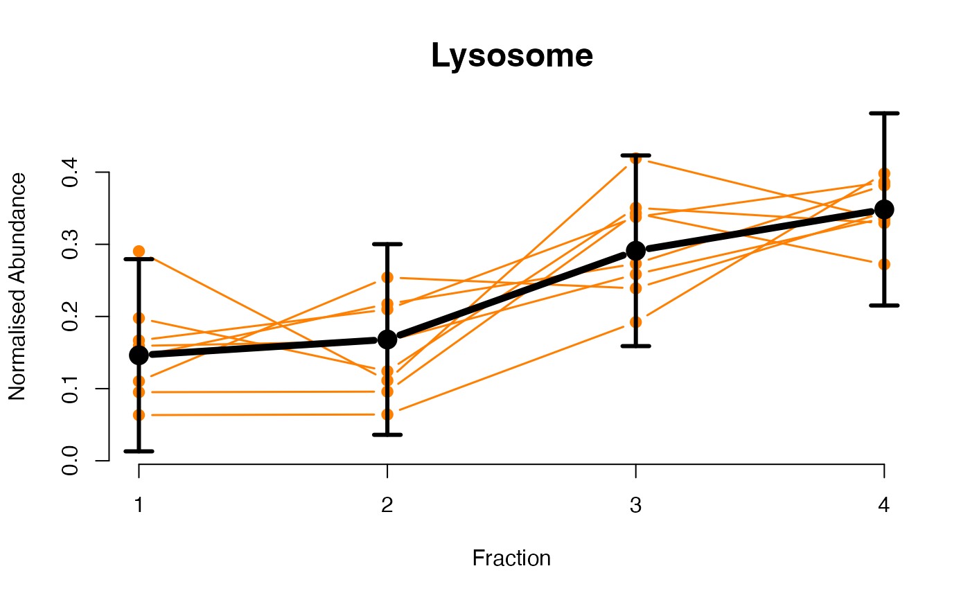
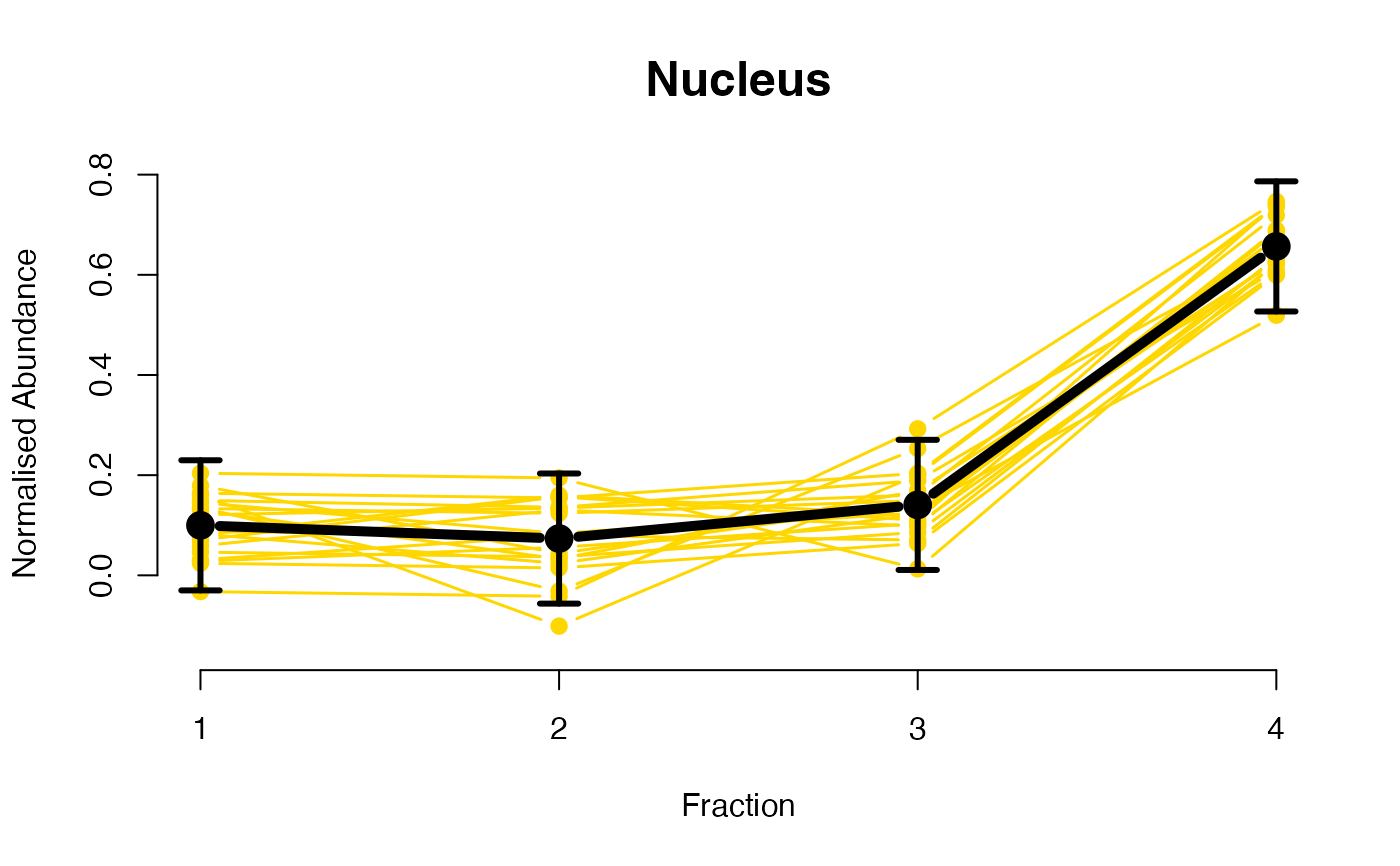
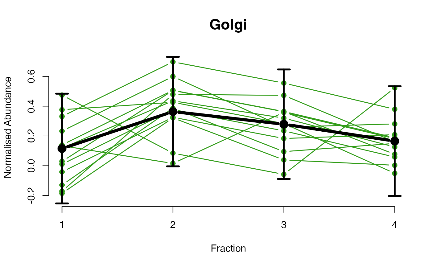
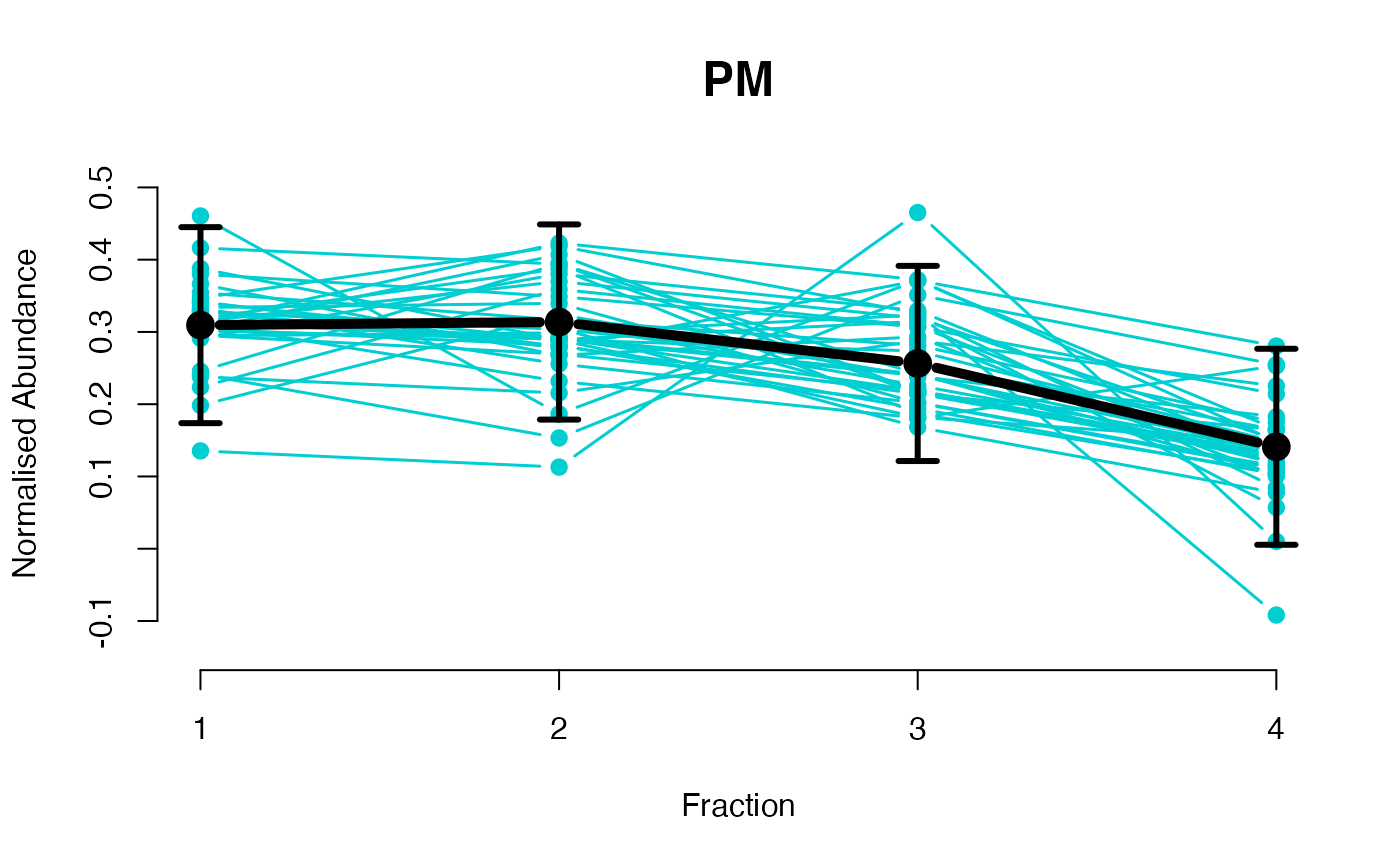
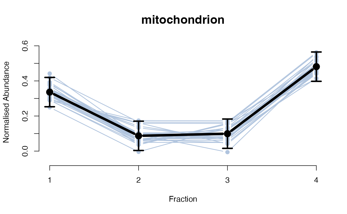
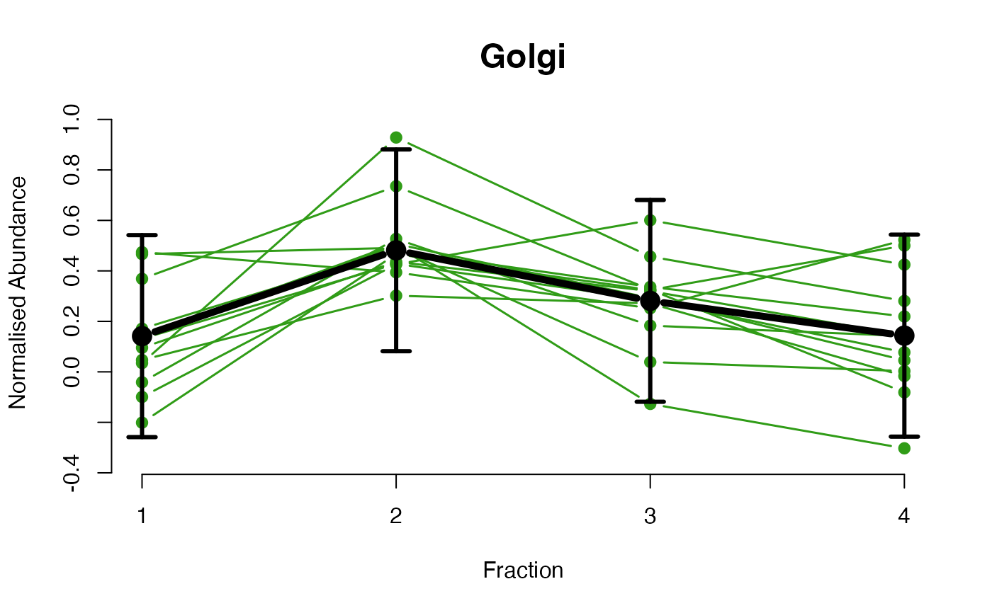
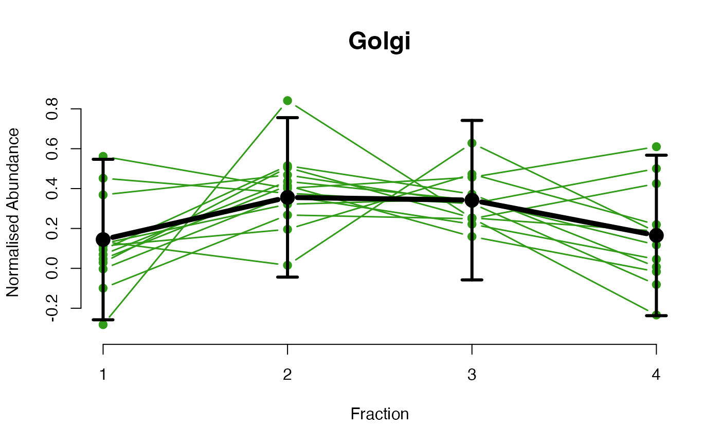
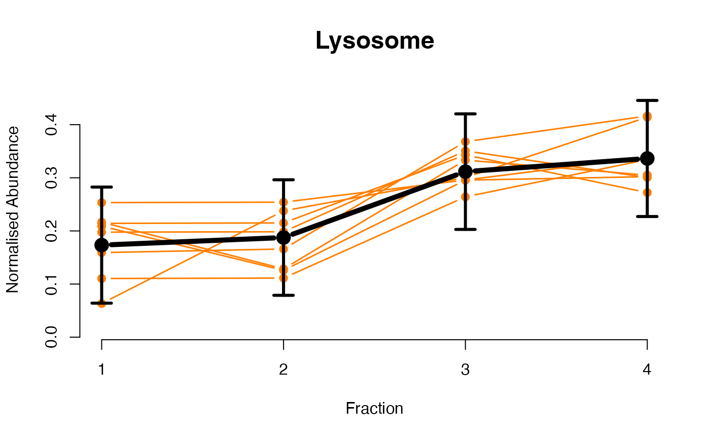
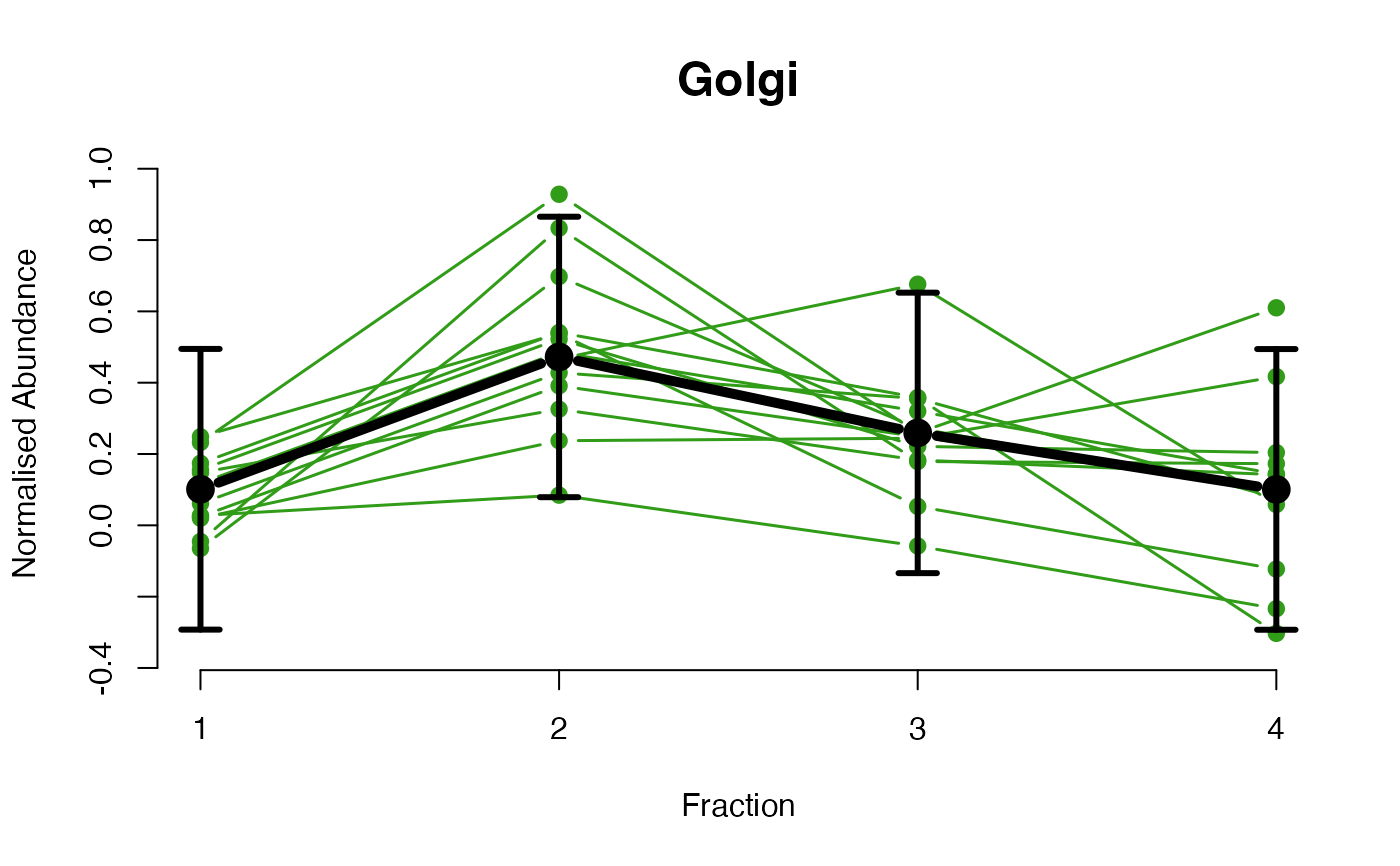
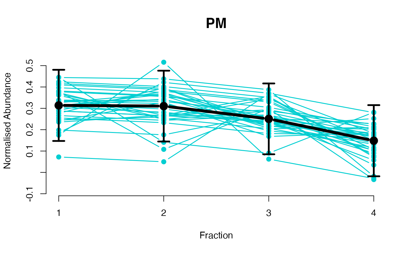
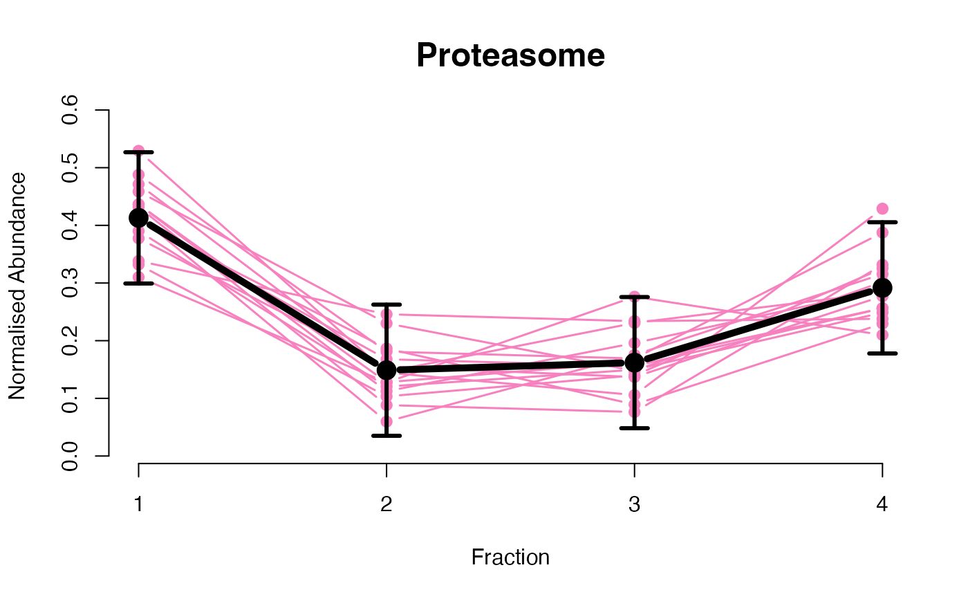
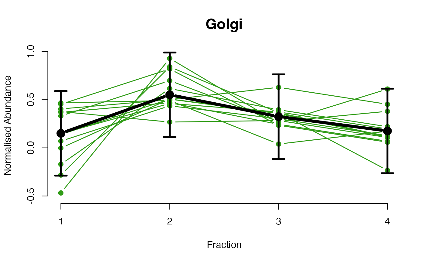
The functions plotGPmatern plot the posterior predictives overlayed with the markers for each subcellular class.

Details

This set of functions allow users to fit GPs to their data. The fitGPmaternPC function allows users to pass a vector of penalised complexity hyperparameters using the hyppar argument. You must provide a matrix with 3 columns and 1 row. The order of these 3 columns represent the hyperparameters length-scale, amplitude, variance. We have found that the matrix(c(10, 60, 250), nrow = 1) worked well for the spatial proteomics datasets tested in Crook et al (2021). This was visually assessed by passing these values and visualising the GP fit using the plotGPmatern function (please see vignette for an example of the output). Generally, (1) increasing the lengthscale parameter (the first column of the hyppar matrix) increases the spread of the covariance i.e. the similarity between points, (2) increasing the amplitude parameter (the second column of the hyppar matrix) increases the maximum value of the covariance and lastly (3) decreasing the variance (third column of the hyppar matrix) reduces the smoothness of the function to allow for local variations. We strongly recommend users start with the recommended parameters and change and assess them as necessary for their dataset by visually evaluating the fit of the GPs using the plotGPmatern function. Please see the vignettes for more details and examples.

Examples

library(pRolocdata)
data("tan2009r1")
set.seed(1)
tansim <- sim_dynamic(object = tan2009r1, 
                    numRep = 6L,
                   numDyn = 100L)
gpParams <- lapply(tansim$lopitrep, function(x) fitGP(x))



































































## ====== fitGPmaternPC =====
library(pRolocdata)
data("tan2009r1")
set.seed(1)
tansim <- sim_dynamic(object = tan2009r1, 
                    numRep = 6L,
                   numDyn = 100L)
## Please note that hyppar should be chosen carefully and tested
## by checking the GP fit with the plotGPmatern function
## (please see details above)
gpParams <- lapply(tansim$lopitrep, 
function(x) fitGPmaternPC(x, hyppar = matrix(c(10, 60, 100), nrow = 1)))

## ====== fitGPmatern =====
library(pRolocdata)
data("tan2009r1")
set.seed(1)
tansim <- sim_dynamic(object = tan2009r1, 
                    numRep = 6L,
                   numDyn = 100L)
gpParams <- lapply(tansim$lopitrep, function(x) fitGPmaternPC(x))

## ====== plotGPmatern =====
## generate example data
library(pRolocdata)
data("tan2009r1")
set.seed(1)
tansim <- sim_dynamic(object = tan2009r1, 
                    numRep = 6L,
                   numDyn = 100L)
## fit a GP
gpParams <- lapply(tansim$lopitrep, function(x) fitGP(x))



































































## Overlay posterior predictives onto profiles
## Dataset1 1
par(mfrow = c(2, 3))
plotGPmatern(tansim$lopitrep[[1]], gpParams[[1]])


## Dataset 2, etc.
par(mfrow = c(2, 3))

plotGPmatern(tansim$lopitrep[[2]], gpParams[[2]])