Function to plot the supervised conformational signature analysis results
plotSCSA.RdFunction to plot the supervised conformational signature analysis results
Arguments
- states.plsda
The OPLS-DA object from the supervisedCSA function
- labels
The labels to use for the plot. Construct labels carefully using example below. The labels should be a data frame with the rownames as the states and the columns as the labels to use for the colouring of the labels.
- whichlabel
The column in the labels to use for the analysis. Default is 1
- values
The values to use for the colouring of the labels. Default is
brewer.pal(n = 8, name = "PRGn")[c(1,8)]and "grey" (for unknown labels)- type
The type of the labels. Default is "catagorical" but could be "continuous". If "continuous" the "Unknown" values should be recorded as NAs.
Value
A ggplot object
Examples
# Construct labels carefully using known properties of the states (Ligands)
# first a catagorical example
library("RexMS")
data("out_lxr_compound_proccessed")
data("LXRalpha_compounds")
states <- names(LXRalpha_compounds)
labels <- data.frame(ABCA1 = rep("Unknown", length(states)),
lipogenic = rep("Unknown", length(states)))
rownames(labels) <- states
labels$ABCA1[rownames(labels) %in% c("LXR.623", "AZ9", "AZ8", "AZ5")] <- "low"
labels$ABCA1[rownames(labels) %in% c("Az1", "AZ2", "AZ3", "AZ4", "AZ6",
"AZ7", "AZ876", "T0.901317", "WAY.254011",
"F1", "GW3965", "BMS.852927")] <- "high"
labels$lipogenic[rownames(labels) %in% c("AZ6", "AZ7", "AZ9",
"AZ8", "GW3965", "BMS.852927",
"LXR.623")] <- "Non-Lipogenic"
labels$lipogenic[rownames(labels) %in% c("AZ876", "AZ1",
"T0.901317", "F1", "WAY.254011")] <- "Lipogenic"
labels$ABCA1 <- factor(labels$ABCA1,
levels = c("low", "high", "Unknown"))
labels$lipogenic <- factor(labels$lipogenic,
levels = c("Non-Lipogenic", "Lipogenic", "Unknown"))
# First using ABCA1 as an example
scsa <- supervisedCSA(RexDifferentialList = out_lxr_compound_proccessed,
quantity = "TRE",
states = states,
labels = labels,
whichlabel = "ABCA1",
whichTimepoint = 600,
orthoI = 1)
#> Warning: OPLS: number of predictive components ('predI' argument) set to 1
#> Warning: The variance of the 263 following variables is less than 2.2e-16 in the full or partial (cross-validation) dataset: these variables will be removed:
#> 1, 2, 3, 4, 5, 6, 7, 8, 9, 10, 11, 12, 13, 14, 15, 16, 17, 18, 19, 20, 21, 22, 23, 24, 25, 26, 27, 28, 29, 30, 31, 32, 33, 34, 35, 36, 37, 38, 39, 40, 41, 42, 43, 44, 45, 46, 47, 48, 49, 50, 51, 52, 53, 54, 55, 56, 57, 58, 59, 60, 61, 62, 63, 64, 65, 66, 67, 68, 69, 70, 71, 72, 73, 74, 75, 76, 77, 78, 79, 80, 81, 82, 83, 84, 85, 86, 87, 88, 89, 90, 91, 92, 93, 94, 95, 96, 97, 98, 99, 100, 101, 102, 103, 104, 105, 106, 107, 108, 109, 110, 111, 112, 113, 114, 115, 116, 117, 118, 119, 120, 121, 122, 123, 124, 125, 126, 127, 128, 129, 130, 131, 132, 133, 134, 135, 136, 137, 138, 139, 140, 141, 142, 143, 144, 145, 146, 147, 148, 149, 150, 151, 152, 153, 154, 155, 156, 157, 158, 159, 160, 161, 162, 163, 164, 165, 166, 167, 168, 169, 170, 171, 172, 173, 174, 175, 176, 177, 178, 179, 180, 181, 182, 183, 184, 185, 186, 187, 188, 189, 190, 191, 192, 193, 194, 195, 196, 197, 198, 199, 200, 201, 204, 208, 214, 215, 234, 235, 237, 239, 242, 244, 258, 259, 260, 261, 262, 268, 272, 276, 279, 280, 291, 300, 308, 317, 318, 319, 320, 332, 333, 334, 335, 336, 338, 342, 350, 357, 358, 359, 360, 361, 366, 370, 390, 391, 392, 393, 394, 395, 396, 397, 398, 399, 400, 401, 402, 403, 404, 405, 406, 428, 436, 437
#> OPLS-DA
#> 14 samples x 184 variables and 1 response
#> standard scaling of predictors and response(s)
#> 263 excluded variables (near zero variance)
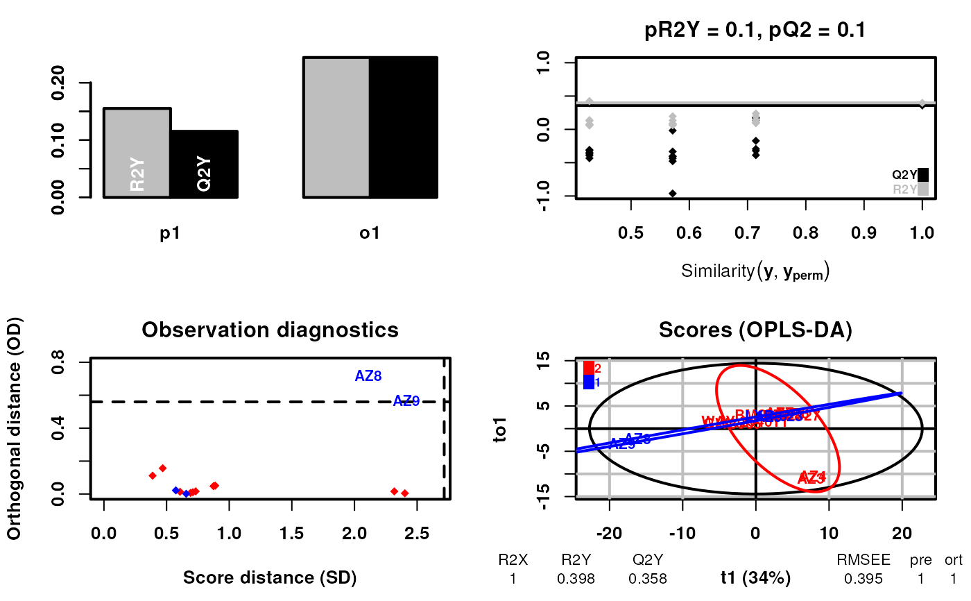
#> R2X(cum) R2Y(cum) Q2(cum) RMSEE pre ort pR2Y pQ2
#> Total 1 0.398 0.358 0.395 1 1 0.1 0.1
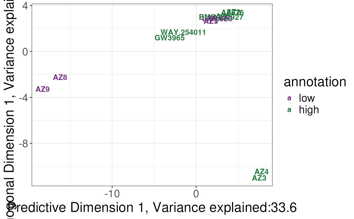
 plotSCSA(states.plsda = scsa,
labels = labels,
whichlabel = "ABCA1")
plotSCSA(states.plsda = scsa,
labels = labels,
whichlabel = "ABCA1")