Differential HDX-MS with RexMS
Oliver Crook
University of Oxfordococrook@gmail.com
2 June 2024
DifferentialRexMS.RmdIntroduction
This vignette demonstrates how to use the RexMS package
to perform differential HDX-MS analysis. We recommend that you start
with the introduction to RexMS vignette first so that you cover the
basics. We skip some of those initial steps here to focus on the aspects
important for differential analysis.
Loading data
We will load the data from the RexMS package. This data
is a subset of the data used in the original publication and focuses on
BRD4 apo and in complex with I-BET151 both datasets are
available as part of the package. Here, we are interested in the changes
in HD exchange as a results of ligand binding. To speed up the analysis
we filter the data to only include the first 100 residues and again
calculate a number of valuable quantities.
require(RexMS)
#> Loading required package: RexMS
#> Loading required package: S4Vectors
#> Loading required package: stats4
#> Loading required package: BiocGenerics
#>
#> Attaching package: 'BiocGenerics'
#> The following objects are masked from 'package:stats':
#>
#>     IQR, mad, sd, var, xtabs
#> The following objects are masked from 'package:base':
#>
#>     anyDuplicated, aperm, append, as.data.frame, basename, cbind,
#>     colnames, dirname, do.call, duplicated, eval, evalq, Filter, Find,
#>     get, grep, grepl, intersect, is.unsorted, lapply, Map, mapply,
#>     match, mget, order, paste, pmax, pmax.int, pmin, pmin.int,
#>     Position, rank, rbind, Reduce, rownames, sapply, setdiff, sort,
#>     table, tapply, union, unique, unsplit, which.max, which.min
#>
#> Attaching package: 'S4Vectors'
#> The following object is masked from 'package:utils':
#>
#>     findMatches
#> The following objects are masked from 'package:base':
#>
#>     expand.grid, I, unname
require(dplyr)
#> Loading required package: dplyr
#>
#> Attaching package: 'dplyr'
#> The following objects are masked from 'package:S4Vectors':
#>
#>     first, intersect, rename, setdiff, setequal, union
#> The following objects are masked from 'package:BiocGenerics':
#>
#>     combine, intersect, setdiff, union
#> The following objects are masked from 'package:stats':
#>
#>     filter, lag
#> The following objects are masked from 'package:base':
#>
#>     intersect, setdiff, setequal, union

data("BRD4_apo")
data("BRD4_ibet")

BRD4_apo <- BRD4_apo %>% filter(End < 100)
BRD4_ibet <- BRD4_ibet %>% filter(End < 100)
numTimepoints <- length(unique(BRD4_apo$Exposure))
Timepoints <- unique(BRD4_apo$Exposure)
numPeptides <- length(unique(BRD4_apo$Sequence))
We actually only need to run rex explicitly on the
condition we are primarily interested in e.g. ‘ligand’ vs ‘apo’, we only
need to model the first dataset initially. If you swap the analysis
around and start with apo first your results will be
inverted (e.g. report protection instead of deprotection) as a
consequence of the data. If you need to separate out conditions from one
csv file it maybe useful to use
filter(State == "my protein state"), where
"my protein state" would be replace by the state you wishes
to extract from the data. The syntax is similar to the filter line used
to extract the first 100 residues.
The following function will run the rex function on the
data in the ligand bound state and then RexProcess will
populate the object as in the original analysis. Again we would
recommend running this function for a much large number of
iterations.
set.seed(1)
rex_ibet <- rex(HdxData = DataFrame(BRD4_ibet),
                numIter = 100,
                R = max(BRD4_ibet$End),
                numtimepoints = numTimepoints,
                timepoints = Timepoints,
                density = "laplace",
                seed = 1L,
                tCoef = c(0, rep(1, 5)),
                BPPARAM = SerialParam())
#> Fold 1 ... Fold 2 ... Fold 3 ... Fold 4 ... Fold 5 ...
#>   |                                                                              |                                                                      |   0%
#> Fold 1 ... Fold 2 ... Fold 3 ... Fold 4 ... Fold 5 ...
#>   |                                                                              |                                                                      |   0%

rex_ibet <- RexProcess(HdxData = DataFrame(BRD4_ibet),
                        params = rex_ibet,
                        range = 50:100,
                        thin = 1,
                        whichChains = c(1,2))
We recommend checking the results as you would in the case of a single-protein analysis but to simplify the analysis we will skip this step here. We plot the sigmas and log-likelihoods for the ligand bound state below.
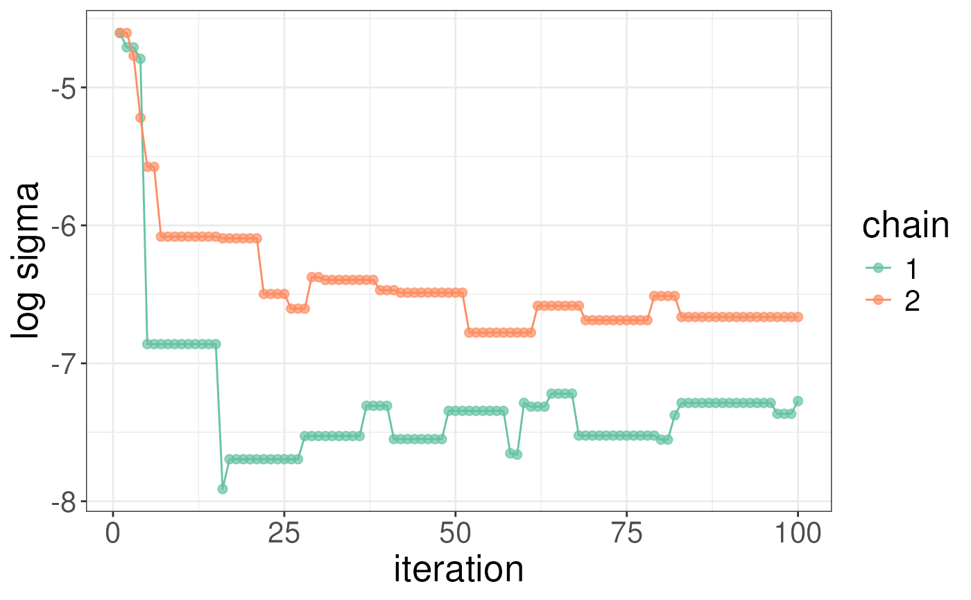
# zoom in on results a bit but adding the lim arguements
plotLogLikelihoods(rex_ibet) + xlim(c(25,100)) + ylim(c(-500,-150))
#> Warning: Removed 48 rows containing missing values or values outside the scale range
#> (`geom_point()`).
#> Warning: Removed 48 rows containing missing values or values outside the scale range
#> (`geom_line()`).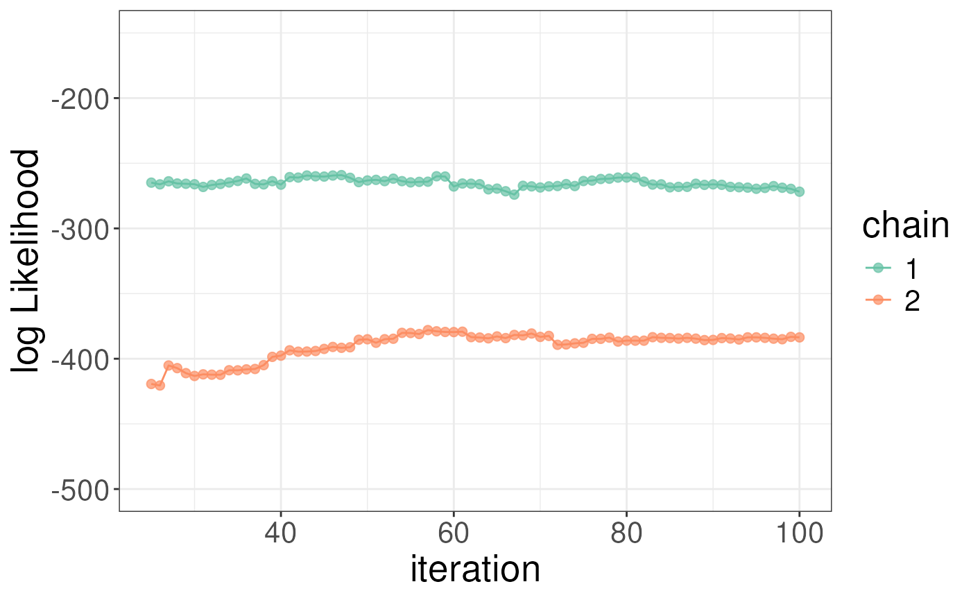 To obtain differential results as compared to the apo (or some other
state) use the following function carefully. In the
To obtain differential results as compared to the apo (or some other
state) use the following function carefully. In the params
argument you want to pass the object that was created by the
rex function for the ibet state. In the
HdxData argument you want to pass the data for the apo
state (or the state you wish to compare to). The whichChain
argument is used to specify which chain you are interested in using to
calculate the differential results. Chain 2 had a higher log-likelihood
in the ligand bound state, so we will use this chain to calculate the
differential results.
rex_diff <- processDifferential(params = rex_ibet,
                                HdxData = DataFrame(BRD4_apo),
                                whichChain = c(2))
This results in an object of class RexDifferential which
has five slots:
- Rex.predictionError - the prediction error for the differential analysis at the level of peptides
- Rex.estimates - the estimates for the differential analysis at the level of residues
- Rex.probs - the probabilities for the differential analysis at the level of residues
- Rex.eFDR - the estimated false discovery rate for the differential analysis at various probability thresholds.
We can access these slots as follows and inspect the object
rex_diff
#>  Object of class "RexDifferential"
Rex.predictionError(rex_diff)
#> DataFrame with 19 rows and 7 columns
#>                    Peptide         0        15        60        600      3600
#>                <character> <numeric> <numeric> <numeric>  <numeric> <numeric>
#> 1   MSAESGPGTRLRNLPVMGDG..         0 -0.414995 -0.420704  1.4592555  2.239965
#> 2   SGPGTRLRNLPVMGDGLETSQM         0 -0.412812 -0.281018  1.3728437  2.114763
#> 3          RNLPVMGDGLETSQM         0 -0.963184 -1.116532  0.0444354  0.623347
#> 4             PVMGDGLETSQM         0  1.477895  1.110257  1.3880638  1.028726
#> 5           STTQAQAQPQPANA         0 -0.626016 -1.044653 -0.6869987 -0.477065
#> ...                    ...       ...       ...       ...        ...       ...
#> 15          QFAWPFQQPVDAVK         0 -0.791349 -1.747475  -2.381059 -1.323146
#> 16              FAWPFQQPVD         0 -0.378110 -0.669854  -1.187098 -1.160246
#> 17           FAWPFQQPVDAVK         0 -0.657529 -1.543422  -2.079057 -1.088530
#> 18                 PFQQPVD         0 -0.105938 -0.268322  -0.447024 -0.446177
#> 19                LNLPDYYK         0 -0.174304 -0.366718  -1.130525 -0.815158
#>         14400
#>     <numeric>
#> 1    1.726412
#> 2    1.728030
#> 3    0.503184
#> 4    0.991215
#> 5   -0.510378
#> ...       ...
#> 15  -1.712488
#> 16  -1.678391
#> 17  -1.427896
#> 18  -0.635282
#> 19  -0.645006
Rex.estimates(rex_diff)
#> DataFrame with 99 rows and 16 columns
#>      Resdiues signedARE_15 signedARE_60 signedARE_600 signedARE_3600
#>     <numeric>    <numeric>    <numeric>     <numeric>      <numeric>
#> 1           1          NaN          NaN           NaN            NaN
#> 2           2          NaN          NaN           NaN            NaN
#> 3           3   -0.0188634   -0.0191229     0.0663298       0.101817
#> 4           4   -0.0188634   -0.0191229     0.0663298       0.101817
#> 5           5   -0.0188634   -0.0191229     0.0663298       0.101817
#> ...       ...          ...          ...           ...            ...
#> 95         95          NaN          NaN           NaN            NaN
#> 96         96   -0.0348608   -0.0733437     -0.226105      -0.163032
#> 97         97   -0.0348608   -0.0733437     -0.226105      -0.163032
#> 98         98   -0.0348608   -0.0733437     -0.226105      -0.163032
#> 99         99   -0.0348608   -0.0733437     -0.226105      -0.163032
#>     signedARE_14400    ARE_15    ARE_60   ARE_600  ARE_3600 ARE_14400
#>           <numeric> <numeric> <numeric> <numeric> <numeric> <numeric>
#> 1               NaN       NaN       NaN       NaN       NaN       NaN
#> 2               NaN       NaN       NaN       NaN       NaN       NaN
#> 3         0.0784733 0.0188634 0.0191229 0.0663298  0.101817 0.0784733
#> 4         0.0784733 0.0188634 0.0191229 0.0663298  0.101817 0.0784733
#> 5         0.0784733 0.0188634 0.0191229 0.0663298  0.101817 0.0784733
#> ...             ...       ...       ...       ...       ...       ...
#> 95              NaN       NaN       NaN       NaN       NaN       NaN
#> 96        -0.129001 0.0348608 0.0733437  0.226105  0.163032  0.129001
#> 97        -0.129001 0.0348608 0.0733437  0.226105  0.163032  0.129001
#> 98        -0.129001 0.0348608 0.0733437  0.226105  0.163032  0.129001
#> 99        -0.129001 0.0348608 0.0733437  0.226105  0.163032  0.129001
#>         TRE_15     TRE_60   TRE_600  TRE_3600 TRE_14400
#>      <numeric>  <numeric> <numeric> <numeric> <numeric>
#> 1    0.0000000  0.0000000 0.0000000  0.000000 0.0000000
#> 2    0.0000000  0.0000000 0.0000000  0.000000 0.0000000
#> 3   -0.0188634 -0.0191229 0.0663298  0.101817 0.0784733
#> 4   -0.0188634 -0.0191229 0.0663298  0.101817 0.0784733
#> 5   -0.0188634 -0.0191229 0.0663298  0.101817 0.0784733
#> ...        ...        ...       ...       ...       ...
#> 95   0.0000000  0.0000000  0.000000  0.000000  0.000000
#> 96  -0.0348608 -0.0733437 -0.226105 -0.163032 -0.129001
#> 97  -0.0348608 -0.0733437 -0.226105 -0.163032 -0.129001
#> 98  -0.0348608 -0.0733437 -0.226105 -0.163032 -0.129001
#> 99  -0.0348608 -0.0733437 -0.226105 -0.163032 -0.129001
Rex.probs(rex_diff)
#> DataFrame with 99 rows and 7 columns
#>      Residues  probs_15  probs_60 probs_600 probs_3600 probs_14400 totalprobs
#>     <numeric> <numeric> <numeric> <numeric>  <numeric>   <numeric>  <numeric>
#> 1           1    0.0000    0.0000    0.0000     0.0000      0.0000   0.000000
#> 2           2    0.0000    0.0000    0.0000     0.0000      0.0000   0.000000
#> 3           3    0.5132    0.5262    0.9320     0.9844      0.9562   0.236905
#> 4           4    0.5384    0.5322    0.9258     0.9830      0.9564   0.249396
#> 5           5    0.5338    0.5360    0.9264     0.9822      0.9534   0.248209
#> ...       ...       ...       ...       ...        ...         ...        ...
#> 95         95    0.0000    0.0000    0.0000     0.0000      0.0000   0.000000
#> 96         96    0.7522    0.9476    1.0000     0.9976      0.9926   0.705812
#> 97         97    0.7456    0.9416    0.9998     0.9986      0.9934   0.696308
#> 98         98    0.7530    0.9450    1.0000     0.9992      0.9952   0.707603
#> 99         99    0.7502    0.9464    1.0000     0.9990      0.9952   0.705875
Rex.eFDR(rex_diff)
#> DataFrame with 100 rows and 6 columns
#>     Threshold    eFDR_15    eFDR_60    eFDR_600  eFDR_3600 eFDR_14400
#>     <numeric>  <numeric>  <numeric>   <numeric>  <numeric>  <numeric>
#> 1        1.00 0.00000000 0.00000000 0.000000000 0.00000000 0.00000000
#> 2        0.99 0.00138333 0.00105000 0.000668571 0.00038500 0.00152195
#> 3        0.98 0.00138333 0.00410435 0.002551220 0.00186364 0.00152195
#> 4        0.97 0.00138333 0.00512500 0.003641860 0.00228000 0.00152195
#> 5        0.96 0.00138333 0.00512500 0.003641860 0.00365106 0.00916154
#> ...       ...        ...        ...         ...        ...        ...
#> 96       0.05   0.230418   0.178537    0.108558   0.148505  0.0364895
#> 97       0.04   0.230418   0.178537    0.108558   0.148505  0.0364895
#> 98       0.03   0.230418   0.178537    0.108558   0.148505  0.0364895
#> 99       0.02   0.230418   0.178537    0.108558   0.148505  0.0364895
#> 100      0.01   0.230418   0.178537    0.108558   0.148505  0.0364895
We can plot the results for the differential analysis as follows. The
following will produce a volcano plot of the results. The
nrow argument specifies the number of row to facet over.
The quantity argument specifies the quantity to plot on the
y-axis. The options are TRE, or ARE. TRE
account for the redundancy at the residue and so is the recommended
option. As we can see from the plot it is very simple to observe the
generaly trend toward protection/stablisation as the small molecules
binds to the protien it will reduce its flexibility.
gg1 <- plotVolcano(diff_params = rex_diff,
nrow = 5,
quantity = "TRE")
gg1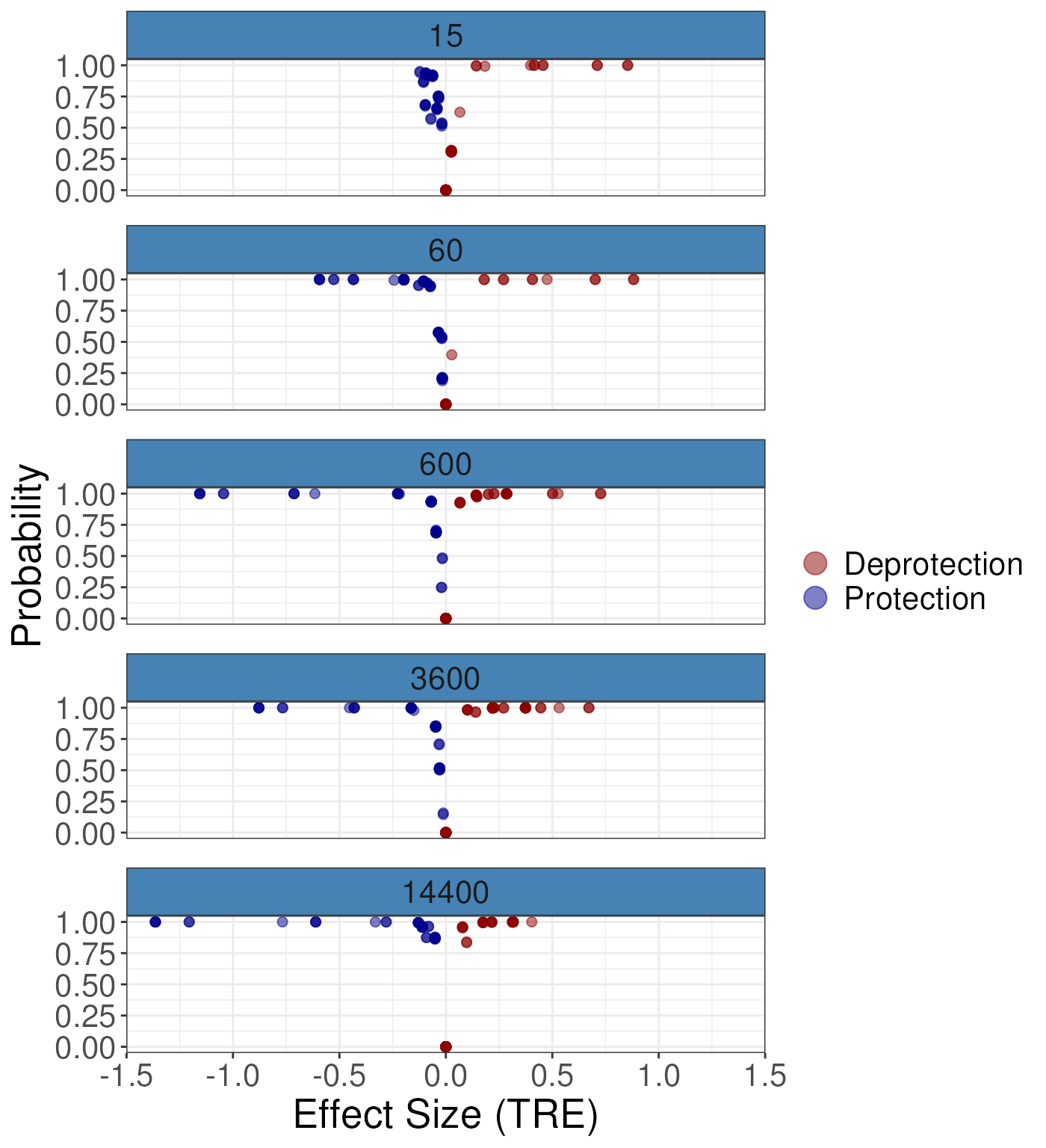 For the ARE:
gg2 <- plotVolcano(diff_params = rex_diff,
                   nrow = 5,
                   quantity = "ARE")
gg2
#> Warning: Removed 230 rows containing missing values or values outside the scale range
#> (`geom_point()`).
To add in the spatial context we suggest a line/butterfly plot:
gg3 <- plotButterfly(diff_params = rex_diff,
                     nrow = 5,
                     quantity = "TRE")

gg3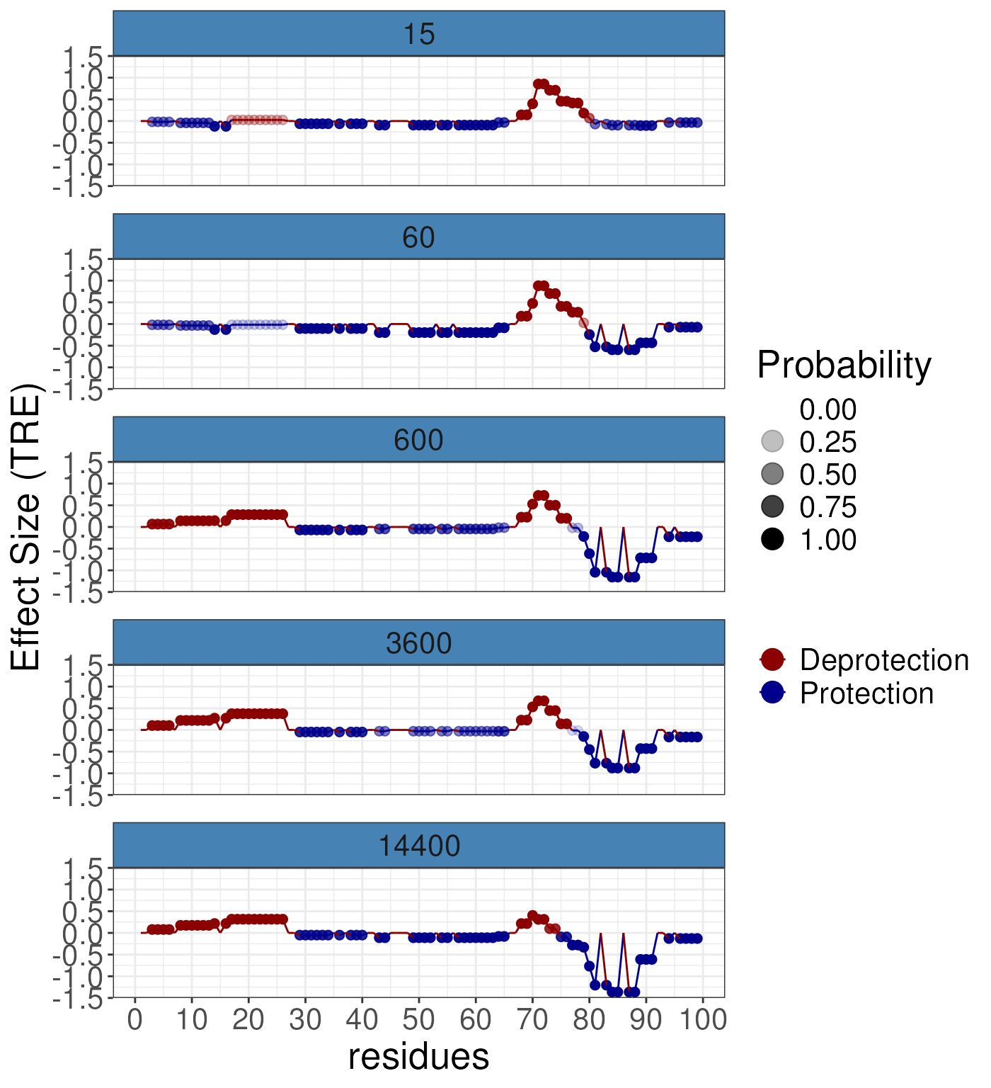
gg3 <- plotButterfly(diff_params = rex_diff,
nrow = 5,
quantity = "signedARE")
gg3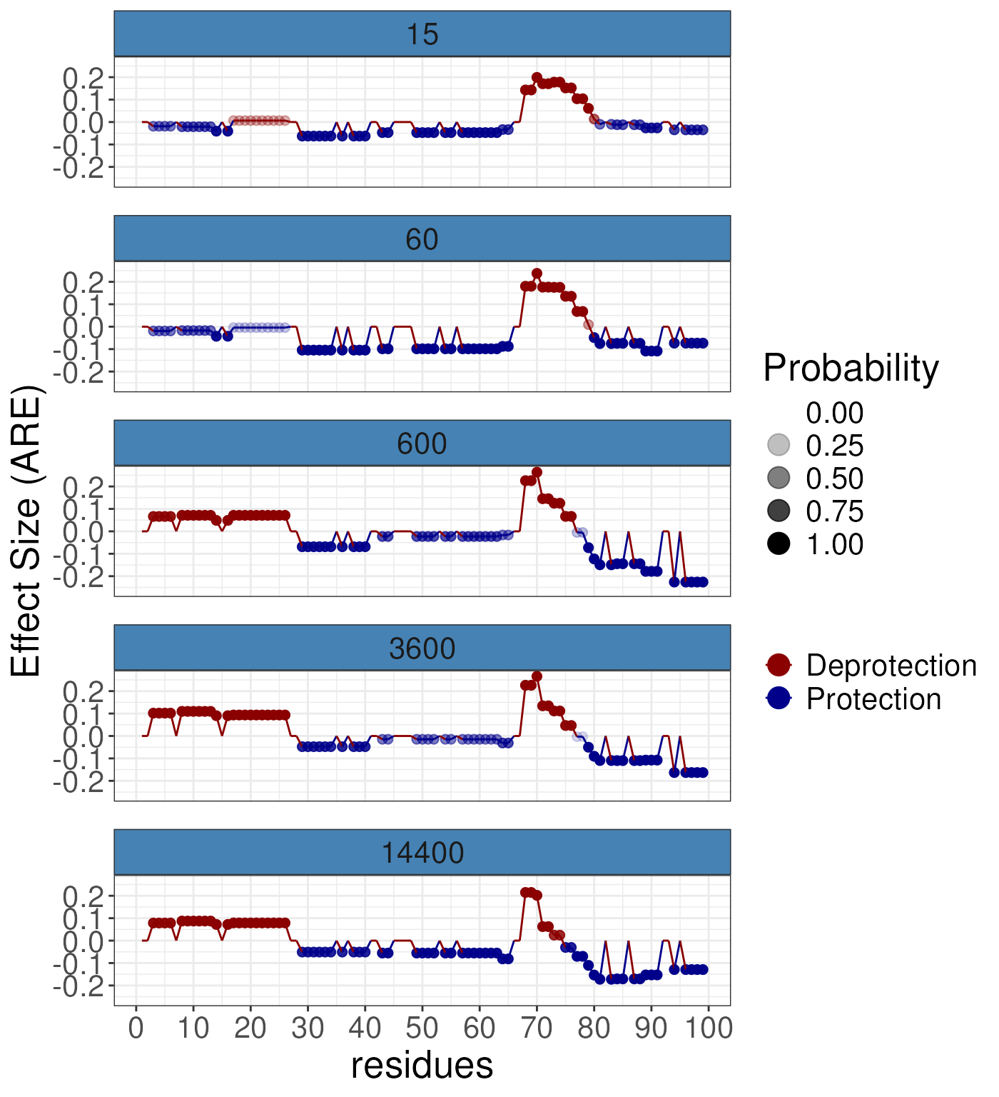 If you wish to average over time then we suggest using the following
function. This will average the results over time and produce a line
plot. This is usually a good way to see that some effects are time
dependent and not supported at all timepoints, whilst for some residues
the effect is consistent across all timepoints.
If you wish to average over time then we suggest using the following
function. This will average the results over time and produce a line
plot. This is usually a good way to see that some effects are time
dependent and not supported at all timepoints, whilst for some residues
the effect is consistent across all timepoints.
gg4 <- plotTimeAveragedButterfly(diff_params = rex_diff)
gg4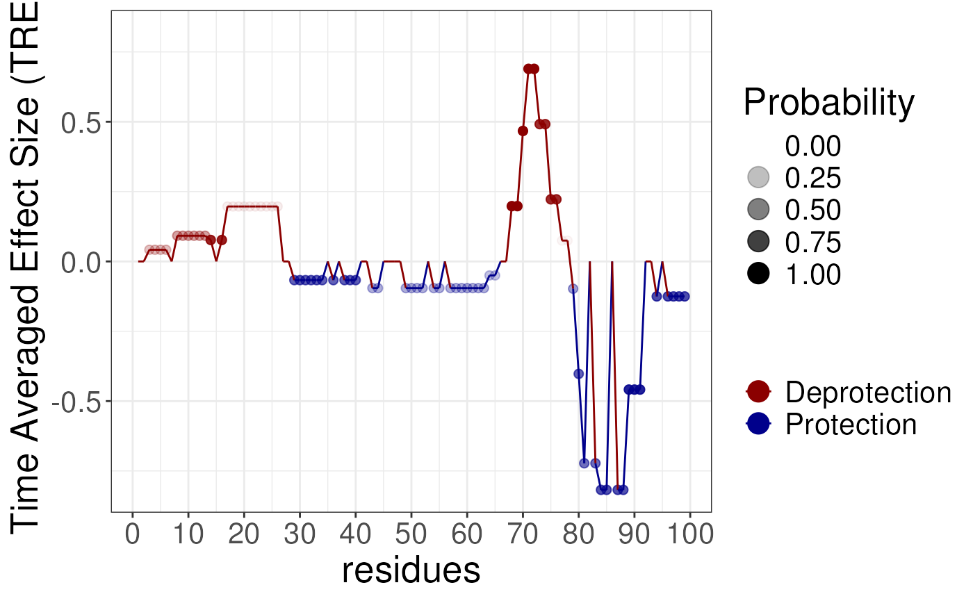 You may also wish to interpret the probabilities carefully and convert
them to an estimated of the expected false discovery rate - i.e. if I
picked a probability threshold what is the predicted number of false
claims I would make. This is stored in the
You may also wish to interpret the probabilities carefully and convert
them to an estimated of the expected false discovery rate - i.e. if I
picked a probability threshold what is the predicted number of false
claims I would make. This is stored in the Rex.eFDR slot.
This will produce a table of the estimated FDR at various probability
thresholds. For example, for a probability threshold of 0.99. The eFDR
for 15 and 60 seconds is not defined (there are no values at this
threshold for these timepoints). The eFDR for 600 second sis 0.00148 or
0.148%, which is quite low. This indicates that if you selected a
probability threshold of 0.99 you would expect to make 0.148% false
claims from claiming a residue was differentially protected/stabilised
when it was not.
Rex.eFDR(rex_diff)
#> DataFrame with 100 rows and 6 columns
#>     Threshold    eFDR_15    eFDR_60    eFDR_600  eFDR_3600 eFDR_14400
#>     <numeric>  <numeric>  <numeric>   <numeric>  <numeric>  <numeric>
#> 1        1.00 0.00000000 0.00000000 0.000000000 0.00000000 0.00000000
#> 2        0.99 0.00138333 0.00105000 0.000668571 0.00038500 0.00152195
#> 3        0.98 0.00138333 0.00410435 0.002551220 0.00186364 0.00152195
#> 4        0.97 0.00138333 0.00512500 0.003641860 0.00228000 0.00152195
#> 5        0.96 0.00138333 0.00512500 0.003641860 0.00365106 0.00916154
#> ...       ...        ...        ...         ...        ...        ...
#> 96       0.05   0.230418   0.178537    0.108558   0.148505  0.0364895
#> 97       0.04   0.230418   0.178537    0.108558   0.148505  0.0364895
#> 98       0.03   0.230418   0.178537    0.108558   0.148505  0.0364895
#> 99       0.02   0.230418   0.178537    0.108558   0.148505  0.0364895
#> 100      0.01   0.230418   0.178537    0.108558   0.148505  0.0364895
RexMS supports transferring these results to protien
structures using the NGLVieweR package. This is a very powerful tool for
visualising the results in the context of the protein structure. The
following code will produce a plot of the protein structure with the
residues coloured by the differential (TRE) results at 15 seconds. The
pdb_filepath argument specifies the path to the pdb file.
The cmap_name argument specifies the name of the colour map
to use. The v argument specifies the values to use for the
colouring. You must provide a local pdb_filepath to use
this function it will not extract the pdb file from the internet.
library(NGLVieweR)
v <- matrix(Rex.estimates(rex_diff)$TRE_15, nrow = 1)
colnames(v) <- seq.int(ncol(v))
v2 <- v[,seq.int(1, 99), drop = FALSE]
colnames(v2) <- seq.int(ncol(v2))

# This complex line is used to get the path to the pdb file from the RexMS package
# yours will probably look like
# pdb_filepath <- "path/to/your/pdb/file.pdb"
pdb_filepath <- system.file("extdata", "test_BRD4.pdb", mustWork = TRUE, package = "RexMS")

mycolor_parameters <- hdx_to_pdb_colours(v2,
                                         pdb = pdb_filepath,
                                         cmap_name = "ProtDeprot")
#> 2024-06-02 13:33:08.540201 [INFO]  Your HDX input dataset has 99 entries
#> 2024-06-02 13:33:08.5405 [INFO]  And excluding NA data you only have 99 entries
#> 2024-06-02 13:33:08.540589 [INFO]  However, your input PDB has only 140 residues in total
#> 2024-06-02 13:33:08.541016 [INFO]  Your scale limits are  -0.12
#>  2024-06-02 13:33:08.541016 [INFO]  Your scale limits are  0.85
#> 2024-06-02 13:33:08.541119 [INFO]  Negative values will be coloured in Blue, and positive ones on Red
view_structure(pdb_filepath = pdb_filepath,
               color_parameters = mycolor_parameters)
You can change the representation if you wish:
view_structure(pdb_filepath = pdb_filepath,
               color_parameters = mycolor_parameters,
               representation = "spacefill")
You can provide any values you would like to colour the structure by. For example using the time-averaged probabilities.
v <- matrix(Rex.probs(rex_diff)$totalprobs, nrow = 1)
colnames(v) <- seq.int(ncol(v))
v2 <- v[,seq.int(1, 99), drop = FALSE]
colnames(v2) <- seq.int(ncol(v2))

mycolor_parameters <- hdx_to_pdb_colours(v2,
                                         pdb = pdb_filepath,
                                         cmap_name = "ProtDeprot")
#> 2024-06-02 13:33:08.739736 [INFO]  Your HDX input dataset has 99 entries
#> 2024-06-02 13:33:08.739847 [INFO]  And excluding NA data you only have 99 entries
#> 2024-06-02 13:33:08.73993 [INFO]  However, your input PDB has only 140 residues in total
#> 2024-06-02 13:33:08.740141 [INFO]  Your scale limits are  0
#>  2024-06-02 13:33:08.740141 [INFO]  Your scale limits are  1
#> 2024-06-02 13:33:08.740224 [INFO]  Negative values will be coloured in Blue, and positive ones on Red
view_structure(pdb_filepath = pdb_filepath,
               color_parameters = mycolor_parameters)
You can also use the viridis colour map if you wish and
plot random colours. The things to remember carefully are match the
residue numbering to your pdb file. If the residue numberings is not the
same as the pdb file you will get incorrect results. This is typical
when expressing a construct of a protein or the structure is only a
small part of the protein.
library(viridis)
#> Loading required package: viridisLite
# random colours
v <- matrix(rnorm(100), nrow = 1)
colnames(v) <- seq.int(ncol(v))
v2 <- v[,seq.int(1, 99), drop = FALSE]
colnames(v2) <- seq.int(ncol(v2))

mycolor_parameters <- hdx_to_pdb_colours(v2,
                                         pdb = pdb_filepath,
                                         cmap_name = "viridis")
#> 2024-06-02 13:33:08.872076 [INFO]  Your HDX input dataset has 99 entries
#> 2024-06-02 13:33:08.872195 [INFO]  And excluding NA data you only have 99 entries
#> 2024-06-02 13:33:08.872286 [INFO]  However, your input PDB has only 140 residues in total
#> 2024-06-02 13:33:08.872518 [INFO]  Your scale limits are  -3.52
#>  2024-06-02 13:33:08.872518 [INFO]  Your scale limits are  2.91
#> 2024-06-02 13:33:08.872614 [INFO]  Your values will be coloured using Viridis
view_structure(pdb_filepath = pdb_filepath,
               color_parameters = mycolor_parameters)
This is the end of this tutorial if you have many states and perhaps even downstream functional outcomes you may wish to visit the next vignette which covers the ideas of a conformational signature analysis (CSA) where you can use unsupervised and supervised learning to characterise the states.
Reproducibility
The RexMS package (ococrook, 2024) was made possible thanks to:
- R (R Core Team, 2024)
- BiocStyle (Oleś, 2023)
- knitr (Xie, 2024)
- RefManageR (McLean, 2017)
- rmarkdown (Allaire, Xie, Dervieux, McPherson, Luraschi, Ushey, Atkins, Wickham, Cheng, Chang, and Iannone, 2024)
- sessioninfo (Wickham, Chang, Flight, Müller, and Hester, 2021)
- testthat (Wickham, 2011)
This package was developed using biocthis.
Date the vignette was generated.
#> [1] "2024-06-02 13:33:09 UTC"Wallclock time spent generating the vignette.
#> Time difference of 2.597 minsR session information.
#> ─ Session info ───────────────────────────────────────────────────────────────────────────────────────────────────────
#>  setting  value
#>  version  R version 4.3.3 (2024-02-29)
#>  os       Ubuntu 22.04.4 LTS
#>  system   x86_64, linux-gnu
#>  ui       X11
#>  language en
#>  collate  en_US.UTF-8
#>  ctype    en_US.UTF-8
#>  tz       UTC
#>  date     2024-06-02
#>  pandoc   3.1.1 @ /usr/local/bin/ (via rmarkdown)
#>
#> ─ Packages ───────────────────────────────────────────────────────────────────────────────────────────────────────────
#>  package              * version    date (UTC) lib source
#>  abind                  1.4-5      2016-07-21 [1] RSPM (R 4.3.0)
#>  backports              1.4.1      2021-12-13 [1] RSPM (R 4.3.0)
#>  bibtex                 0.5.1      2023-01-26 [1] RSPM (R 4.3.0)
#>  bio3d                  2.4-4      2022-10-26 [1] RSPM (R 4.3.0)
#>  Biobase                2.62.0     2023-10-24 [1] Bioconductor
#>  BiocGenerics         * 0.48.1     2023-11-01 [1] Bioconductor
#>  BiocManager            1.30.22    2023-08-08 [1] RSPM (R 4.3.0)
#>  BiocParallel           1.36.0     2023-10-24 [1] Bioconductor
#>  BiocStyle            * 2.30.0     2023-10-24 [1] Bioconductor
#>  bitops                 1.0-7      2021-04-24 [1] RSPM (R 4.3.0)
#>  bookdown               0.39       2024-04-15 [1] RSPM (R 4.3.0)
#>  bslib                  0.7.0      2024-03-29 [2] RSPM (R 4.3.0)
#>  cachem                 1.0.8      2023-05-01 [2] RSPM (R 4.3.0)
#>  calibrate              1.7.7      2020-06-19 [1] RSPM (R 4.3.0)
#>  cli                    3.6.2      2023-12-11 [2] RSPM (R 4.3.0)
#>  cluster                2.1.6      2023-12-01 [3] CRAN (R 4.3.3)
#>  coda                   0.19-4.1   2024-01-31 [1] RSPM (R 4.3.0)
#>  codetools              0.2-20     2024-03-31 [3] RSPM (R 4.3.0)
#>  colorspace             2.1-0      2023-01-23 [1] RSPM (R 4.3.0)
#>  comprehenr             0.6.10     2021-01-31 [1] RSPM (R 4.3.0)
#>  crayon                 1.5.2      2022-09-29 [2] RSPM (R 4.3.0)
#>  DBI                    1.2.2      2024-02-16 [1] RSPM (R 4.3.0)
#>  dbplyr                 2.5.0      2024-03-19 [1] RSPM (R 4.3.0)
#>  DelayedArray           0.28.0     2023-10-24 [1] Bioconductor
#>  desc                   1.4.3      2023-12-10 [2] RSPM (R 4.3.0)
#>  digest                 0.6.35     2024-03-11 [2] RSPM (R 4.3.0)
#>  dplyr                * 1.1.4      2023-11-17 [1] RSPM (R 4.3.0)
#>  evaluate               0.23       2023-11-01 [2] RSPM (R 4.3.0)
#>  fansi                  1.0.6      2023-12-08 [2] RSPM (R 4.3.0)
#>  farver                 2.1.1      2022-07-06 [1] RSPM (R 4.3.0)
#>  fastmap                1.1.1      2023-02-24 [2] RSPM (R 4.3.0)
#>  fs                     1.6.3      2023-07-20 [2] RSPM (R 4.3.0)
#>  generics               0.1.3      2022-07-05 [1] RSPM (R 4.3.0)
#>  genlasso               1.6.1      2022-08-22 [1] RSPM (R 4.3.0)
#>  GenomeInfoDb           1.38.8     2024-03-15 [1] Bioconductor 3.18 (R 4.3.2)
#>  GenomeInfoDbData       1.2.11     2024-04-06 [1] Bioconductor
#>  GenomicRanges          1.54.1     2023-10-29 [1] Bioconductor
#>  ggplot2              * 3.5.0      2024-02-23 [1] RSPM (R 4.3.0)
#>  glue                   1.7.0      2024-01-09 [2] RSPM (R 4.3.0)
#>  gridExtra              2.3        2017-09-09 [1] RSPM (R 4.3.0)
#>  gtable                 0.3.5      2024-04-22 [1] RSPM (R 4.3.0)
#>  highr                  0.10       2022-12-22 [2] RSPM (R 4.3.0)
#>  htmltools              0.5.8.1    2024-04-04 [2] RSPM (R 4.3.0)
#>  htmlwidgets            1.6.4      2023-12-06 [2] RSPM (R 4.3.0)
#>  httpuv                 1.6.15     2024-03-26 [2] RSPM (R 4.3.0)
#>  httr                   1.4.7      2023-08-15 [2] RSPM (R 4.3.0)
#>  igraph                 2.0.3      2024-03-13 [1] RSPM (R 4.3.0)
#>  IRanges                2.36.0     2023-10-24 [1] Bioconductor
#>  jquerylib              0.1.4      2021-04-26 [2] RSPM (R 4.3.0)
#>  jsonlite               1.8.8      2023-12-04 [2] RSPM (R 4.3.0)
#>  knitr                  1.46       2024-04-06 [2] RSPM (R 4.3.0)
#>  labeling               0.4.3      2023-08-29 [1] RSPM (R 4.3.0)
#>  LaplacesDemon          16.1.6     2021-07-09 [1] RSPM (R 4.3.0)
#>  later                  1.3.2      2023-12-06 [2] RSPM (R 4.3.0)
#>  lattice                0.22-6     2024-03-20 [3] RSPM (R 4.3.0)
#>  lifecycle              1.0.4      2023-11-07 [2] RSPM (R 4.3.0)
#>  limma                  3.58.1     2023-10-31 [1] Bioconductor
#>  lubridate              1.9.3      2023-09-27 [1] RSPM (R 4.3.0)
#>  magrittr               2.0.3      2022-03-30 [2] RSPM (R 4.3.0)
#>  MASS                   7.3-60.0.1 2024-01-13 [3] CRAN (R 4.3.3)
#>  Matrix                 1.6-5      2024-01-11 [3] CRAN (R 4.3.3)
#>  MatrixGenerics         1.14.0     2023-10-24 [1] Bioconductor
#>  matrixStats            1.3.0      2024-04-11 [1] RSPM (R 4.3.0)
#>  memoise                2.0.1      2021-11-26 [2] RSPM (R 4.3.0)
#>  mgcv                   1.9-1      2023-12-21 [3] CRAN (R 4.3.3)
#>  mime                   0.12       2021-09-28 [2] RSPM (R 4.3.0)
#>  minpack.lm             1.2-4      2023-09-11 [1] RSPM (R 4.3.0)
#>  MultiAssayExperiment   1.28.0     2023-10-24 [1] Bioconductor
#>  MultiDataSet           1.30.0     2023-10-24 [1] Bioconductor
#>  munsell                0.5.1      2024-04-01 [1] RSPM (R 4.3.0)
#>  NGLVieweR            * 1.3.1      2021-06-01 [1] RSPM (R 4.3.0)
#>  nlme                   3.1-164    2023-11-27 [3] CRAN (R 4.3.3)
#>  permute                0.9-7      2022-01-27 [1] RSPM (R 4.3.0)
#>  pheatmap               1.0.12     2019-01-04 [1] RSPM (R 4.3.0)
#>  pillar                 1.9.0      2023-03-22 [2] RSPM (R 4.3.0)
#>  pkgconfig              2.0.3      2019-09-22 [2] RSPM (R 4.3.0)
#>  pkgdown                2.0.9      2024-04-18 [2] RSPM (R 4.3.0)
#>  plyr                   1.8.9      2023-10-02 [1] RSPM (R 4.3.0)
#>  promises               1.3.0      2024-04-05 [2] RSPM (R 4.3.0)
#>  purrr                  1.0.2      2023-08-10 [2] RSPM (R 4.3.0)
#>  qqman                  0.1.9      2023-08-23 [1] RSPM (R 4.3.0)
#>  R6                     2.5.1      2021-08-19 [2] RSPM (R 4.3.0)
#>  ragg                   1.3.0      2024-03-13 [2] RSPM (R 4.3.0)
#>  RColorBrewer           1.1-3      2022-04-03 [1] RSPM (R 4.3.0)
#>  Rcpp                   1.0.12     2024-01-09 [2] RSPM (R 4.3.0)
#>  RCurl                  1.98-1.14  2024-01-09 [1] RSPM (R 4.3.0)
#>  RefManageR           * 1.4.0      2022-09-30 [1] RSPM (R 4.3.0)
#>  RexMS                * 0.99.7     2024-06-02 [1] Bioconductor
#>  rlang                  1.1.3      2024-01-10 [2] RSPM (R 4.3.0)
#>  rlog                   0.1.0      2021-02-24 [1] RSPM (R 4.3.0)
#>  rmarkdown              2.26       2024-03-05 [2] RSPM (R 4.3.0)
#>  ropls                  1.34.0     2023-10-24 [1] Bioconductor
#>  S4Arrays               1.2.1      2024-03-04 [1] Bioconductor 3.18 (R 4.3.2)
#>  S4Vectors            * 0.40.2     2023-11-23 [1] Bioconductor 3.18 (R 4.3.2)
#>  sass                   0.4.9      2024-03-15 [2] RSPM (R 4.3.0)
#>  scales                 1.3.0      2023-11-28 [1] RSPM (R 4.3.0)
#>  sessioninfo          * 1.2.2      2021-12-06 [2] RSPM (R 4.3.0)
#>  shiny                  1.8.1.1    2024-04-02 [2] RSPM (R 4.3.0)
#>  SparseArray            1.2.4      2024-02-11 [1] Bioconductor 3.18 (R 4.3.2)
#>  statmod                1.5.0      2023-01-06 [1] RSPM (R 4.3.0)
#>  stringi                1.8.3      2023-12-11 [2] RSPM (R 4.3.0)
#>  stringr                1.5.1      2023-11-14 [2] RSPM (R 4.3.0)
#>  SummarizedExperiment   1.32.0     2023-10-24 [1] Bioconductor
#>  systemfonts            1.0.6      2024-03-07 [2] RSPM (R 4.3.0)
#>  textshaping            0.3.7      2023-10-09 [2] RSPM (R 4.3.0)
#>  tibble                 3.2.1      2023-03-20 [2] RSPM (R 4.3.0)
#>  tidyr                  1.3.1      2024-01-24 [1] RSPM (R 4.3.0)
#>  tidyselect             1.2.1      2024-03-11 [1] RSPM (R 4.3.0)
#>  timechange             0.3.0      2024-01-18 [1] RSPM (R 4.3.0)
#>  utf8                   1.2.4      2023-10-22 [2] RSPM (R 4.3.0)
#>  vctrs                  0.6.5      2023-12-01 [2] RSPM (R 4.3.0)
#>  vegan                  2.6-4      2022-10-11 [1] RSPM (R 4.3.0)
#>  viridis              * 0.6.5      2024-01-29 [1] RSPM (R 4.3.0)
#>  viridisLite          * 0.4.2      2023-05-02 [1] RSPM (R 4.3.0)
#>  withr                  3.0.0      2024-01-16 [2] RSPM (R 4.3.0)
#>  xfun                   0.43       2024-03-25 [2] RSPM (R 4.3.0)
#>  xml2                   1.3.6      2023-12-04 [2] RSPM (R 4.3.0)
#>  xtable                 1.8-4      2019-04-21 [2] RSPM (R 4.3.0)
#>  XVector                0.42.0     2023-10-24 [1] Bioconductor
#>  yaml                   2.3.8      2023-12-11 [2] RSPM (R 4.3.0)
#>  zlibbioc               1.48.2     2024-03-13 [1] Bioconductor 3.18 (R 4.3.2)
#>
#>  [1] /__w/_temp/Library
#>  [2] /usr/local/lib/R/site-library
#>  [3] /usr/local/lib/R/library
#>
#> ──────────────────────────────────────────────────────────────────────────────────────────────────────────────────────
Bibliography
This vignette was generated using BiocStyle (Oleś, 2023) with knitr (Xie, 2024) and rmarkdown (Allaire, Xie, Dervieux et al., 2024) running behind the scenes.
Citations made with RefManageR (McLean, 2017).
[1] J. Allaire, Y. Xie, C. Dervieux, et al. rmarkdown: Dynamic Documents for R. R package version 2.26. 2024. URL: https://github.com/rstudio/rmarkdown.
[2] M. W. McLean. “RefManageR: Import and Manage BibTeX and BibLaTeX References in R”. In: The Journal of Open Source Software (2017). DOI: 10.21105/joss.00338.
[3] ococrook. Inferring residue level hydrogen deuterium exchange with ReX. https://github.com/ococrook/ReX/ReX - R package version 0.99.7. 2024. DOI: 10.18129/B9.bioc.ReX. URL: http://www.bioconductor.org/packages/ReX.
[4] A. Oleś. BiocStyle: Standard styles for vignettes and other Bioconductor documents. R package version 2.30.0. 2023. DOI: 10.18129/B9.bioc.BiocStyle. URL: https://bioconductor.org/packages/BiocStyle.
[5] R Core Team. R: A Language and Environment for Statistical Computing. R Foundation for Statistical Computing. Vienna, Austria, 2024. URL: https://www.R-project.org/.
[6] H. Wickham. “testthat: Get Started with Testing”. In: The R Journal 3 (2011), pp. 5–10. URL: https://journal.r-project.org/archive/2011-1/RJournal_2011-1_Wickham.pdf.
[7] H. Wickham, W. Chang, R. Flight, et al. sessioninfo: R Session Information. R package version 1.2.2, https://r-lib.github.io/sessioninfo/. 2021. URL: https://github.com/r-lib/sessioninfo#readme.
[8] Y. Xie. knitr: A General-Purpose Package for Dynamic Report Generation in R. R package version 1.46. 2024. URL: https://yihui.org/knitr/.