Conformational Signature Analysis
Oliver Crook
University of Oxfordococrook@gmail.com
2 June 2024
ConformationalSignatureAnalysis.RmdIntroduction
This vignette explains how to perform conformational signature analysis (CSA). The essential idea is when you have an experimental design in which you have numerous states (such as ligand binding, mutants, antibodies) and in each state you performed HDX-MS and potentially measured a downstream outcome. You can use conformational signature analysis to identify the regions of the protein that are most likely to be associated for the observed outcome. This can then inform design choices. There are three options currently implemented:
Unsupervised Conformational Signature Analysis - This is the most basic form of the analysis. It will identify the regions of the protein that are most variable across the states. This is useful for identifying regions that are associated with the variation in the data. By performing the analysis in this way you will identify the states that are most similar and different from each other.
Supervised Conformational Signature Analysis with discrete outcomes - This is a more advanced form of the analysis using a discrete outcome (such as “monovalent” or “antagonist”). It will identify the regions of the protein that are most variable across the states and are also associated with the outcome. This is useful for identifying regions that are associated with the outcome. This is done by dimensionality reduction that accounts for the outcome.
Supervised Conformational Signature Analysis with continuous outcomes - This is a more advanced form of the analysis using a continuous outcome such as binding affinity. It will identify the regions of the protein that are most variable across the states and are also associated with the outcome. This is useful for identifying regions that are associated with the outcome. This is done by dimensionality reduction that accounts for the continuous outcome.
The analysis currently supports missing values in the outcomes but not the HDX-MS data.
The trickest part of the analysis is setting up the data correctly. You can do this in a excel file and load as csv but we will demonstrate using R manually below. Essentially you want to create a dataset where the rownames are the different states and columns indicate the labels associated with the states.
Getting started
First, we will load the library and the data. The data is a list of dataframes where each dataframe is a state. Each dataframe should have the following columns
- Sequence - The peptide sequence
- Start - The start of the peptide
- End - The end of the peptide
- Exposure - The timepoint of the HDX-MS experiment
- Uptake - The deuteration of the peptide
- State - The state of the HDX-MS experiment
- MaxUptake - The maximum deuteration of the peptide
- replicate - The replicate of the HDX-MS experiment
This is as in the single protein analysis. We suggest performing that analysis carefully, first, before proceeding to the conformational signature analysis. We recommend storing the reference or apo state in a separate dataframe. The analysis expects consistency between the experiments (e.g. replicates and number of timepoints, region of the protein) but you do not need to measure the exact same peptides in each experiment. You will also need to name the states you are interested in and store them in a vector.
library(RexMS)## Loading required package: S4Vectors## Loading required package: stats4## Loading required package: BiocGenerics##
## Attaching package: 'BiocGenerics'## The following objects are masked from 'package:stats':
##
## IQR, mad, sd, var, xtabs## The following objects are masked from 'package:base':
##
## anyDuplicated, aperm, append, as.data.frame, basename, cbind,
## colnames, dirname, do.call, duplicated, eval, evalq, Filter, Find,
## get, grep, grepl, intersect, is.unsorted, lapply, Map, mapply,
## match, mget, order, paste, pmax, pmax.int, pmin, pmin.int,
## Position, rank, rbind, Reduce, rownames, sapply, setdiff, sort,
## table, tapply, union, unique, unsplit, which.max, which.min##
## Attaching package: 'S4Vectors'## The following object is masked from 'package:utils':
##
## findMatches## The following objects are masked from 'package:base':
##
## expand.grid, I, unname
# for conformation signature analysis organise data into a list

data("LXRalpha_compounds") # data for different compounds as a list
data("LXRalpha_processed") # data for the reference state

# usual important terms
numTimepoints <- length(unique(LXRalpha_compounds[[1]]$Exposure))
Timepoints <- unique(LXRalpha_compounds[[1]]$Exposure)
numPeptides <- length(unique(LXRalpha_compounds[[1]]$Sequence))
R <- max(LXRalpha_compounds[[1]]$End)

# names of compounds
states <- names(LXRalpha_compounds)

# let look at states
states
## [1] "T0.091317" "WAY.254011" "F1" "AZ876" "AZ1"
## [6] "AZ2" "AZ3" "AZ4" "GW3965" "BMS.852927"
## [11] "AZ6" "AZ7" "LXR.623" "AZ8" "AZ9"
## [16] "AZ5" "X24.25EC"Our analysis has 18 compounds and a reference state. We will use the
reference state as the reference for the conformational signature
analysis. Whichever route you follow (e.g. supervised or unsupervised)
the initial steps are identical. We will start with the list in an
lapply function. To each element in this list (which is an
entire HDX dataset) we apply the rex function. This
function will perform the usual rex model. There are only 3 timepoints
in this analysis so we will set the tCoef to
c(0, 1, 1). We will also set the seed to 1 for
reproducibility. We will use the SerialParam for the
BPPARAM argument. This is because the analysis is not too
computationally intensive but if you run for many iterations and chains
we suggest using parrallel processing. We will store the results in a
list. For brevity we will run the analysis for 100 iterations but we
recommend much more (typically 5000) for final analysis. The following
function takes a while to run so we will not run them here but pre-load
the results from the package the code is placed for completeness.
set.seed(1)
rex_lxr <- lapply(LXRalpha_compounds, function(xx) {

                rex(HdxData = DataFrame(xx),
                        numIter = 100,
                        R = R,
                        numtimepoints = numTimepoints,
                        timepoints = Timepoints,
                        density = "laplace",
                        seed = 1L,
                        tCoef = c(0, rep(1, 2)),
                        BPPARAM = SerialParam())})
The next step is to apply RexProcess to the output of
the rex function. Remember there are 18 compounds so we
will use lapply again. We will set the range to 50:100 -
removing the first 50 as burnin, though we would typically recommend you
run about 5000 iterations. This is mcmc iteration we are interested in.
We will store the results in a list. Again, we do not actually run the
code here but pre-load the results from the package.
rex_lxr <- lapply(seq_along(rex_lxr),
                            function(i)
                              RexProcess(HdxData = DataFrame(LXRalpha_compounds[[i]]),
                                          params = rex_lxr[[i]],
                                         range = 50:100))
We will now load the results from the package. The results are stored
in the rex_lxr object.
data("rex_lxr")In the next step we would perform the same differential analysis as
in the differential analysis tutorial but 18 times because there are 18
compounds. We will use the same reference state for each compound. We
will store the results in a list. Again, we do not actually run the code
here but pre-load the results from the package. Remember
params are the various states and the HdxData
is the reference state HDX data. The params is the output
of the rex function, which has been processed. The
whichChain is the chain of the analysis you are interested
in using to generate the results. We will use chain 1, but recommend
assessing the quality of multiple chains.
out_lxr_compound_proccessed <- lapply(rex_lxr, function(xx)
                                        processDifferential(HdxData =  DataFrame(LXRalpha_processed),
                                                            params = xx,
                                                            whichChain = 1))
We will now load the results from the package. The results are stored
in the out_lxr_compound_proccessed object.
data("out_lxr_compound_proccessed")Unsupervised Conformational Signature Analysis
To perform the unsupervised conformational signature analysis, we
will use the unsupervisedCSA function. This function will
take the output of the processDifferential function. Whilst
for unsupervised analysis you do not need to specify the outcome, we
will generate the labels results anyway to highlight the details of
setting up that analysis.
For our protein there are 18 compounds and a reference state. Each of the compounds induce one outcome in two scenarios or the outcome is unknown (which is allowed in our analysis). We will generate the labels for the outcomes. We will store the results in a dataframe with the states as the rownames. For proteins where the outcome is unknown, we will set the outcome to “Unknown”. For the two scenarios, the first is ABCA1 induction and the second is lipogencity. We will set the outcome to “low” or “high” for ABCA1 induction. We will set the outcome to “Non-Lipogenic” or “Lipogenic” for lipogenicity. Of course, you may adapt these outcomes to your own analysis. We will then convert the outcomes to factors with the levels in the order we are interested in. You can of course load this dataframe from something that was made in excel and covert to a dataframe.
# First set up the dataframe with unknowns and correct rownames
labels <- data.frame(ABCA1 = rep("Unknown", length(states)),
                     lipogenic = rep("Unknown", length(states)))
rownames(labels) <- states

# Now set the outcomes with ABCA1 induction
labels$ABCA1[rownames(labels) %in% c("LXR.623", "AZ9", "AZ8", "AZ5")] <- "low"
labels$ABCA1[rownames(labels) %in% c("Az1", "AZ2", "AZ3", "AZ4", "AZ6",
                                     "AZ7", "AZ876", "T0.901317", "WAY.254011",
                                     "F1", "GW3965", "BMS.852927")] <- "high"

# Now set the outcomes with lipogenicity
labels$lipogenic[rownames(labels) %in% c("AZ6", "AZ7", "AZ9",
                                         "AZ8", "GW3965", "BMS.852927",
                                                 "LXR.623")] <- "Non-Lipogenic"

labels$lipogenic[rownames(labels) %in% c("AZ876", "AZ1",
                                         "T0.901317", "F1", "WAY.254011")] <- "Lipogenic"

# Now convert to factors with the correct levels
labels$ABCA1 <- factor(labels$ABCA1,
                       levels = c("low", "high", "Unknown"))
labels$lipogenic <- factor(labels$lipogenic,
                           levels = c("Non-Lipogenic", "Lipogenic", "Unknown"))
We will now run the unsupervised conformational signature analysis.
We will set the quantity to “TRE” as this is the quantity
we use to generate the signature. We will set the states to
the states we are interested in. We will set the
whichTimepoint to 600. This is the timepoint used to
generate the conformational signature. We will store the results in the
ucsa object. Since this is the unsupervised analysis, we do
not need to specify the labels argument.
ucsa <- UnsupervisedCSA(RexDifferentialList = out_lxr_compound_proccessed,
                        quantity = "TRE",
                        states = states,
                        whichTimepoint = 600)
We will now look at the results. The results are stored in a list
with the first entry pca_states being the Principal
Component Analysis of the RexMS results. The rotation
matrix can be used as the conformational signature - providing the modes
of conformational variation in the data. This contains all the results
from a PCA analysis. The second entry states_wide is a
dataframe with the states as the columns and the residue as the rows.
The values are the TRE values that were used to generate the
conformational signature.
You can perform any downstream analysis you would like with the
results. For example, you could plot the PCA results. We will plot the
first two components of the PCA analysis. The labels are not used unless
you pass them to the pca_params argument even if you supply
a labels argument.
Note that the results look strange because we have not run the algorithm for enough iterations.
## Loading required package: ggplot2
# doesn't use the labels even though they are passed as an argument
plotUCSA(pca_states = ucsa$pca_states,
         states_wide = ucsa$states_wide,
         labels = labels)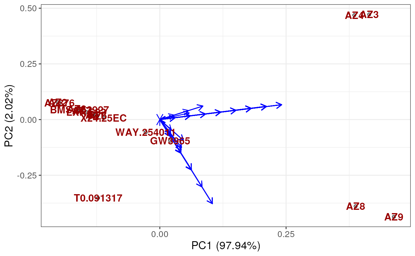
# uses labels to colour the points
plotUCSA(pca_states = ucsa$pca_states,
         states_wide = ucsa$states_wide,
         labels = labels,
         pca_params = list(x = 1, # pca component 1 on x-axis
                           y = 2, # pca component 2 on y-axis
                           whichlabel = "ABCA1")) # colour by ABCA1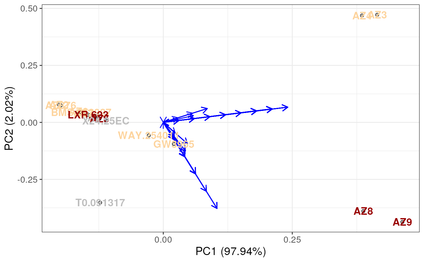
Supervised Conformational Signature Analysis with discrete outcomes
Until now, we have not used the labels as part of the analysis - only to interpret the results of the unsupervised analysis. Supervised conformational signature analysis is more advanced and uses the labels to generate the conformational signature. The idea is to identify the regions of the protein that are most variable across the states and are also associated with the outcome.
To perform the supervised conformational signature analysis with
discrete outcomes, we will use the supervisedCSA function.
This function will take the output of the
processDifferential function. We will generate the labels
for the outcomes as before. We will store the results in a dataframe
with the states as the rownames. For proteins where the outcome is
unknown, we will set the outcome to “Unknown”. For the two scenarios,
the first is ABCA1 induction and the second is lipogencity. We will set
the outcome to “low” or “high” for ABCA1 induction. We will set the
outcome to “Non-Lipogenic” or “Lipogenic” for lipogenicity. Of course,
you may adapt these outcomes to your own analysis. We will then convert
the outcomes to factors with the levels in the order we are interested
in. You can of course load this dataframe from something that was made
in excel and covert to a dataframe.
We will now run the supervised conformational signature analysis with
discrete outcomes. We will set the quantity to “TRE” as
this is the quantity we use to generate the signature. We will set the
states to the states we are interested in. We will set the
whichTimepoint to 600. This is the timepoint used to
generate the conformational signature. We will store the results in the
scsa object. We will set the whichlabel to
“ABCA1” as this is the outcome we are interested in. We will also set
whichlabel to “lipogenic” to generate the conformational
signature for lipogenicity. Since this is the supervised analysis we
need to specify the labels argument from the dataframe we
generated earlier. We will set the orthoI to 1. This is the
number of orthogonal components to use in the analysis. We will set this
to 1 for simplicity. We will store the results in the scsa
object.
The analysis used the labels to generate the conformational signature
by using orthogonal partial least squares discrimant analysis (OPLS-DA).
The results return a formal opls object. This object
contains the results of the analysis.
Note that the results look strange because we have not run the algorith for enough iterations earlier. The results are allowed to contain “Unknown” outcomes.
Note that the algorithm will output a number of warnings - the first is that the number of predictive components is set to 1. This is the desire behaviour. The second is that the variance in some residue elements is below machine precision. This is typical for residues that were not measure in the analysis or where the uptake was 0 (such as Prolines). You do not need to worry about this as the sequence labelling is handled behind the scenes.
scsa <- supervisedCSA(RexDifferentialList = out_lxr_compound_proccessed,
                      quantity = "TRE",
                      states = states,
                      labels = labels,
                      whichlabel = "ABCA1",
                      whichTimepoint = 600,
                      orthoI = 1)
## Warning: OPLS: number of predictive components ('predI' argument) set to 1## Warning: The variance of the 263 following variables is less than 2.2e-16 in the full or partial (cross-validation) dataset: these variables will be removed:
## 1, 2, 3, 4, 5, 6, 7, 8, 9, 10, 11, 12, 13, 14, 15, 16, 17, 18, 19, 20, 21, 22, 23, 24, 25, 26, 27, 28, 29, 30, 31, 32, 33, 34, 35, 36, 37, 38, 39, 40, 41, 42, 43, 44, 45, 46, 47, 48, 49, 50, 51, 52, 53, 54, 55, 56, 57, 58, 59, 60, 61, 62, 63, 64, 65, 66, 67, 68, 69, 70, 71, 72, 73, 74, 75, 76, 77, 78, 79, 80, 81, 82, 83, 84, 85, 86, 87, 88, 89, 90, 91, 92, 93, 94, 95, 96, 97, 98, 99, 100, 101, 102, 103, 104, 105, 106, 107, 108, 109, 110, 111, 112, 113, 114, 115, 116, 117, 118, 119, 120, 121, 122, 123, 124, 125, 126, 127, 128, 129, 130, 131, 132, 133, 134, 135, 136, 137, 138, 139, 140, 141, 142, 143, 144, 145, 146, 147, 148, 149, 150, 151, 152, 153, 154, 155, 156, 157, 158, 159, 160, 161, 162, 163, 164, 165, 166, 167, 168, 169, 170, 171, 172, 173, 174, 175, 176, 177, 178, 179, 180, 181, 182, 183, 184, 185, 186, 187, 188, 189, 190, 191, 192, 193, 194, 195, 196, 197, 198, 199, 200, 201, 204, 208, 214, 215, 234, 235, 237, 239, 242, 244, 258, 259, 260, 261, 262, 268, 272, 276, 279, 280, 291, 300, 308, 317, 318, 319, 320, 332, 333, 334, 335, 336, 338, 342, 350, 357, 358, 359, 360, 361, 366, 370, 390, 391, 392, 393, 394, 395, 396, 397, 398, 399, 400, 401, 402, 403, 404, 405, 406, 428, 436, 437## OPLS-DA
## 14 samples x 184 variables and 1 response
## standard scaling of predictors and response(s)
## 263 excluded variables (near zero variance)
## R2X(cum) R2Y(cum) Q2(cum) RMSEE pre ort pR2Y pQ2
## Total 1 0.398 0.358 0.395 1 1 0.15 0.1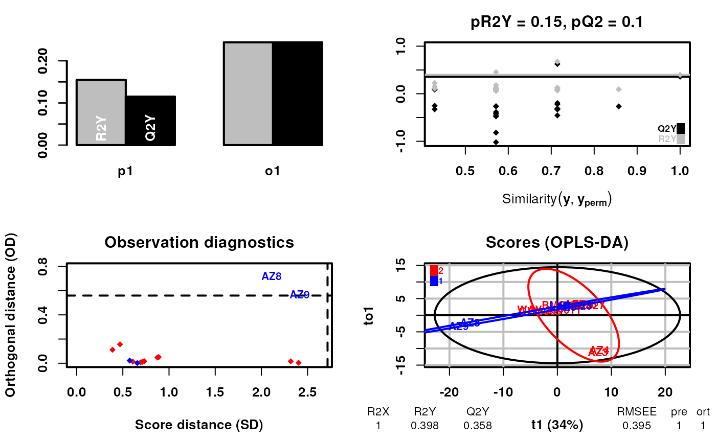
scsa2 <- supervisedCSA(RexDifferentialList = out_lxr_compound_proccessed,
quantity = "TRE",
states = states,
labels = labels,
whichlabel = "lipogenic",
whichTimepoint = 600,
orthoI = 1,
type = "catagorical")## Warning: OPLS: number of predictive components ('predI' argument) set to 1
## Warning: The variance of the 263 following variables is less than 2.2e-16 in the full or partial (cross-validation) dataset: these variables will be removed:
## 1, 2, 3, 4, 5, 6, 7, 8, 9, 10, 11, 12, 13, 14, 15, 16, 17, 18, 19, 20, 21, 22, 23, 24, 25, 26, 27, 28, 29, 30, 31, 32, 33, 34, 35, 36, 37, 38, 39, 40, 41, 42, 43, 44, 45, 46, 47, 48, 49, 50, 51, 52, 53, 54, 55, 56, 57, 58, 59, 60, 61, 62, 63, 64, 65, 66, 67, 68, 69, 70, 71, 72, 73, 74, 75, 76, 77, 78, 79, 80, 81, 82, 83, 84, 85, 86, 87, 88, 89, 90, 91, 92, 93, 94, 95, 96, 97, 98, 99, 100, 101, 102, 103, 104, 105, 106, 107, 108, 109, 110, 111, 112, 113, 114, 115, 116, 117, 118, 119, 120, 121, 122, 123, 124, 125, 126, 127, 128, 129, 130, 131, 132, 133, 134, 135, 136, 137, 138, 139, 140, 141, 142, 143, 144, 145, 146, 147, 148, 149, 150, 151, 152, 153, 154, 155, 156, 157, 158, 159, 160, 161, 162, 163, 164, 165, 166, 167, 168, 169, 170, 171, 172, 173, 174, 175, 176, 177, 178, 179, 180, 181, 182, 183, 184, 185, 186, 187, 188, 189, 190, 191, 192, 193, 194, 195, 196, 197, 198, 199, 200, 201, 204, 208, 214, 215, 234, 235, 237, 239, 242, 244, 258, 259, 260, 261, 262, 268, 272, 276, 279, 280, 291, 300, 308, 317, 318, 319, 320, 332, 333, 334, 335, 336, 338, 342, 350, 357, 358, 359, 360, 361, 366, 370, 390, 391, 392, 393, 394, 395, 396, 397, 398, 399, 400, 401, 402, 403, 404, 405, 406, 428, 436, 437
## OPLS-DA
## 11 samples x 184 variables and 1 response
## standard scaling of predictors and response(s)
## 263 excluded variables (near zero variance)
## R2X(cum) R2Y(cum) Q2(cum) RMSEE pre ort pR2Y pQ2
## Total 1 0.12 -0.0506 0.529 1 1 0.95 0.4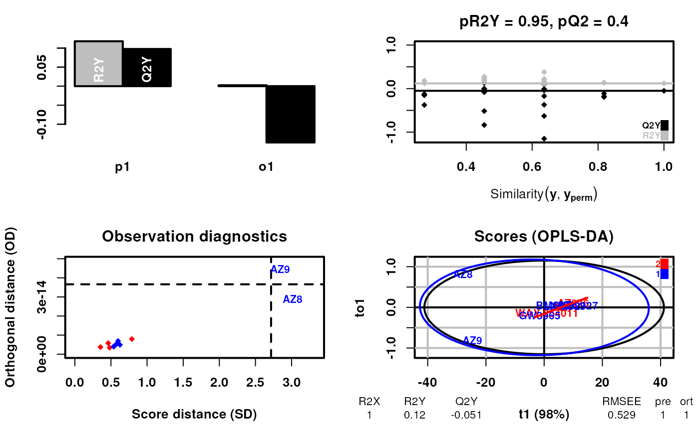
We can now look at the results of the analysis. The results are
stored in the opls object. For each analysis, we can plot
the loading of the conformational signature. This is the regions of the
protein that are most variable across the states and are also associated
with the outcome. We will plot the loadings of the outcomes. The
predictive component is the component that is associated with the
outcome. The orthogonal component is the component that is not
associated with the outcome. We will plot the loadings for ABCA1 and
lipogenicity for both predictive and orthogonal components.
Note again the results look strange because we have not run the algorithm for enough iterations earlier.
plotLoadingSCSA(states.plsda = scsa,
                labels = labels,
                whichLoading = "predictive",
                whichlabel = "ABCA1")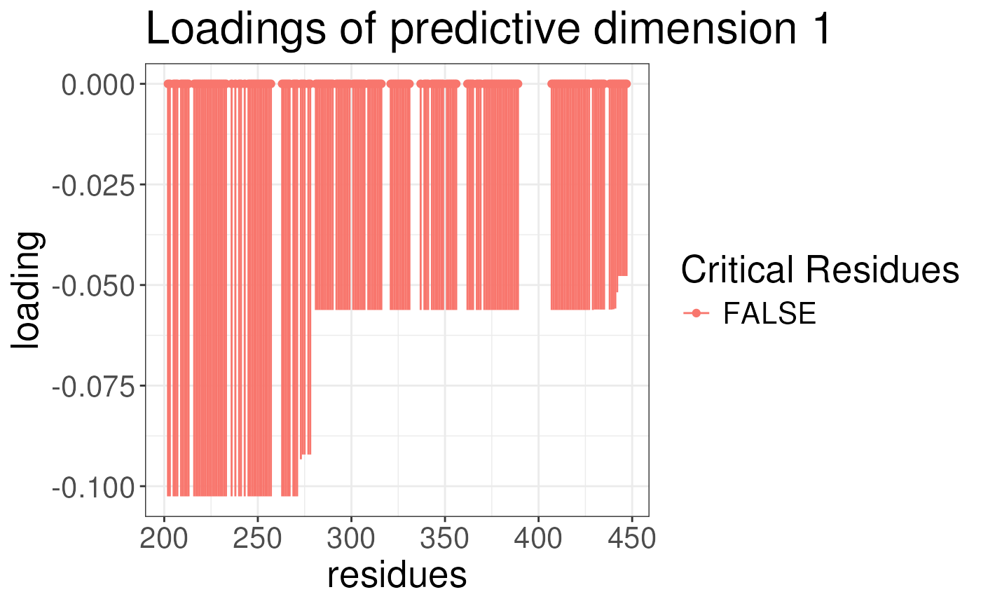
plotLoadingSCSA(states.plsda = scsa,
                labels = labels,
                whichLoading = "orthogonal",
                whichlabel = "ABCA1")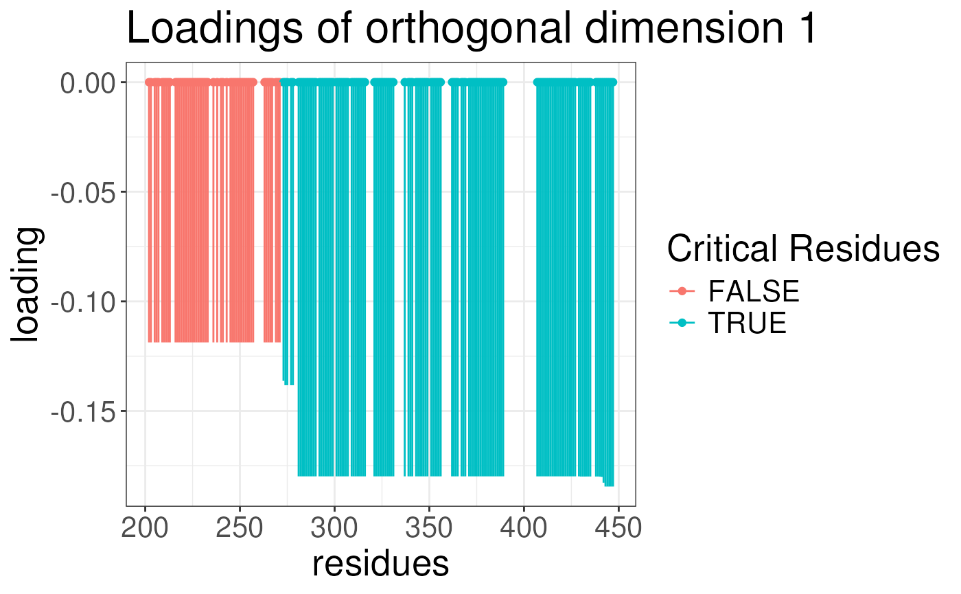
plotLoadingSCSA(states.plsda = scsa2,
                labels = labels,
                whichLoading = "predictive",
                whichlabel = "lipogenic")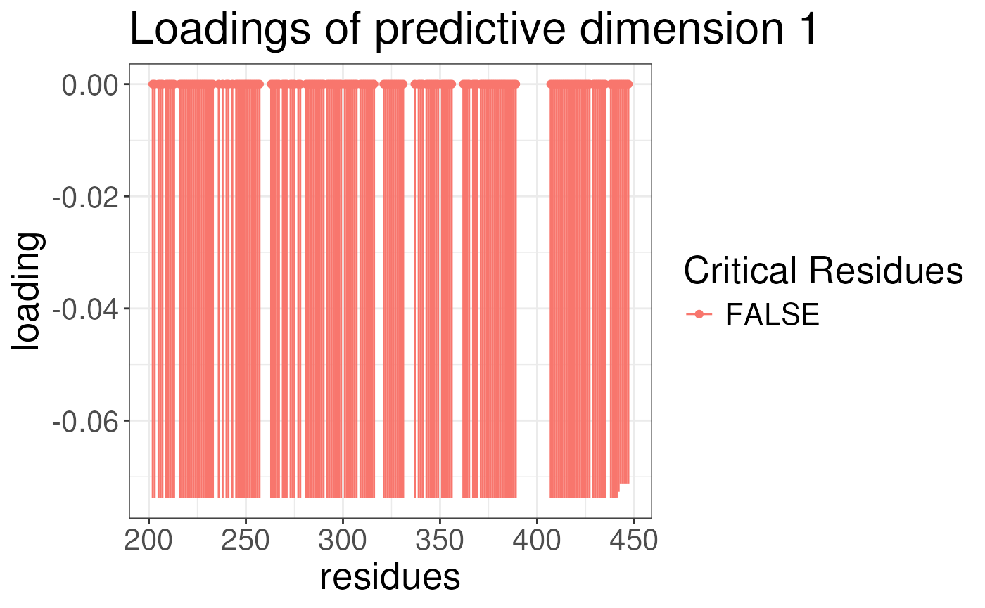
plotLoadingSCSA(states.plsda = scsa2,
                labels = labels,
                whichLoading = "orthogonal",
                whichlabel = "lipogenic")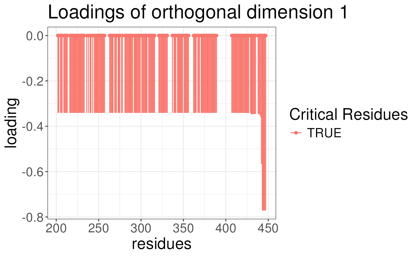
You can also plot the scores of the conformational signature. This is the scores of the samples from the predictive and orthogonal components. We will plot the scores for ABCA1 and lipogenicity for both predictive and orthogonal components.
plotSCSA(states.plsda = scsa2,
         labels = labels,
         whichlabel = "lipogenic")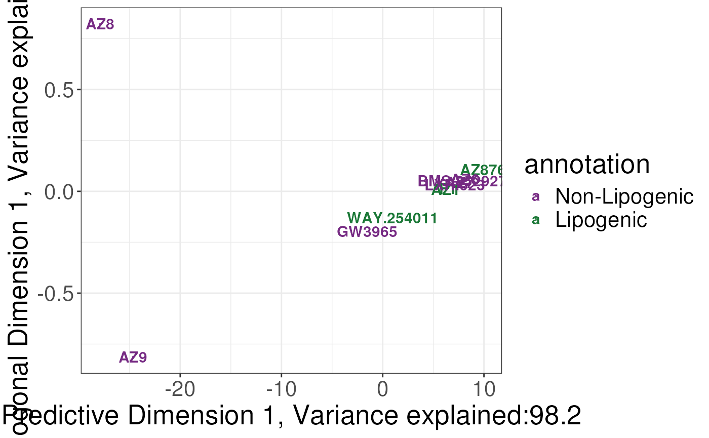
Supervised Conformational Signature Analysis with continuous outcomes
We can also perform the supervised conformational signature analysis
with continuous outcomes. This is similar to the discrete outcomes but
the outcome is continuous. To specify the labels we will generate the
labels for the outcomes as before. We will store the results in a
dataframe with the states as the rownames. For proteins where the
outcome is unknown, we will set the outcome to NA. In this
case, we will use the ED50 as the outcome. We will log the
ED50 values. You can of course load this dataframe from
something that was made in excel and covert to a dataframe. We keep
these values as numeric rather than factors.
labels$ED50 <- NA
labels[, "ED50"] <- log(c(4.11, NA, NA, 0.956, NA, 9.64, 1.49,
                      5.65, 0.969, 2.10, 11.3, NA, 31.5, 341, 32.2, 17.2, NA))
We will now run the supervised conformational signature analysis with
continuous outcomes. We will set the quantity to “TRE” as
this is the quantity we use to generate the signature. We will set the
states to the states we are interested in. We will set the
whichTimepoint to 600. This is the timepoint used to
generate the conformational signature.
To perform the supervised conformational signature analysis with
continuous outcomes, we will use the supervisedCSA
function. In this case, we will set the type to
“continuous” so that it does not perform a discrete analysis. We will
set the whichlabel to “ED50” as this is the outcome we are
interested in.
scsa3 <- supervisedCSA(RexDifferentialList = out_lxr_compound_proccessed,
                      quantity = "TRE",
                      states = states,
                      labels = labels,
                      whichlabel = "ED50",
                      whichTimepoint = 600,
                      orthoI = 1,
                      type = "continuous")
## Warning: OPLS: number of predictive components ('predI' argument) set to 1## Warning: The variance of the 263 following variables is less than 2.2e-16 in the full or partial (cross-validation) dataset: these variables will be removed:
## 1, 2, 3, 4, 5, 6, 7, 8, 9, 10, 11, 12, 13, 14, 15, 16, 17, 18, 19, 20, 21, 22, 23, 24, 25, 26, 27, 28, 29, 30, 31, 32, 33, 34, 35, 36, 37, 38, 39, 40, 41, 42, 43, 44, 45, 46, 47, 48, 49, 50, 51, 52, 53, 54, 55, 56, 57, 58, 59, 60, 61, 62, 63, 64, 65, 66, 67, 68, 69, 70, 71, 72, 73, 74, 75, 76, 77, 78, 79, 80, 81, 82, 83, 84, 85, 86, 87, 88, 89, 90, 91, 92, 93, 94, 95, 96, 97, 98, 99, 100, 101, 102, 103, 104, 105, 106, 107, 108, 109, 110, 111, 112, 113, 114, 115, 116, 117, 118, 119, 120, 121, 122, 123, 124, 125, 126, 127, 128, 129, 130, 131, 132, 133, 134, 135, 136, 137, 138, 139, 140, 141, 142, 143, 144, 145, 146, 147, 148, 149, 150, 151, 152, 153, 154, 155, 156, 157, 158, 159, 160, 161, 162, 163, 164, 165, 166, 167, 168, 169, 170, 171, 172, 173, 174, 175, 176, 177, 178, 179, 180, 181, 182, 183, 184, 185, 186, 187, 188, 189, 190, 191, 192, 193, 194, 195, 196, 197, 198, 199, 200, 201, 204, 208, 214, 215, 234, 235, 237, 239, 242, 244, 258, 259, 260, 261, 262, 268, 272, 276, 279, 280, 291, 300, 308, 317, 318, 319, 320, 332, 333, 334, 335, 336, 338, 342, 350, 357, 358, 359, 360, 361, 366, 370, 390, 391, 392, 393, 394, 395, 396, 397, 398, 399, 400, 401, 402, 403, 404, 405, 406, 428, 436, 437## OPLS
## 12 samples x 184 variables and 1 response
## standard scaling of predictors and response(s)
## 263 excluded variables (near zero variance)
## R2X(cum) R2Y(cum) Q2(cum) RMSEE pre ort pR2Y pQ2
## Total 0.997 0.363 0.0176 1.52 1 1 0.15 0.3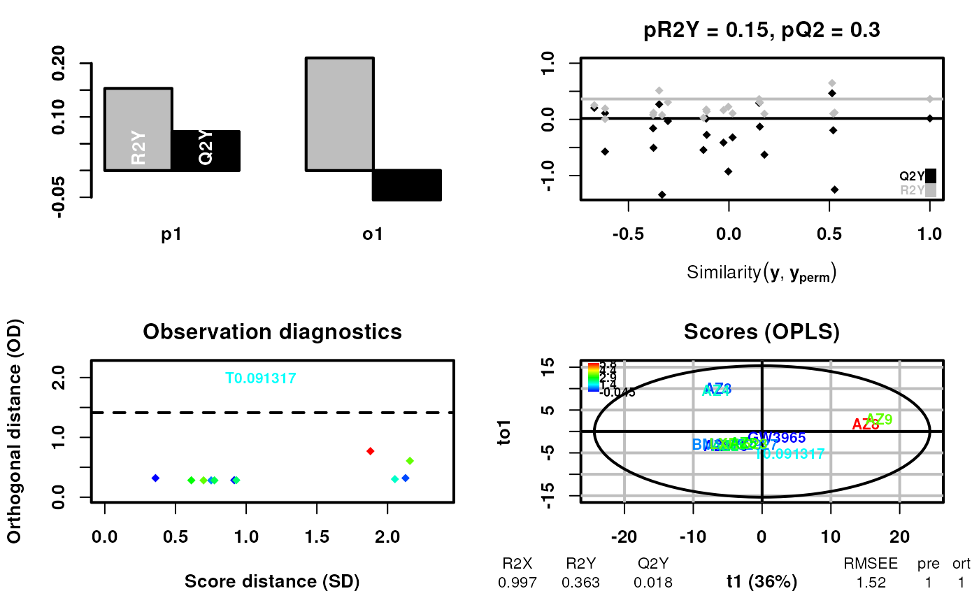
We can now look at the results of the analysis. The results are
stored in the opls object. We can plot the loading of the
conformational signature. This is the regions of the protein that are
most variable across the states and are also associated with the
outcome. We will also plot the scores of the conformational signature.
This is the scores of the samples on the predictive and orthogonal
components. We will plot the loadings and scores for the
ED50 outcome.
plotSCSA(states.plsda = scsa3,
         labels = labels,
         whichlabel = "ED50",
         type = "continuous") + labs(col = "log ED50")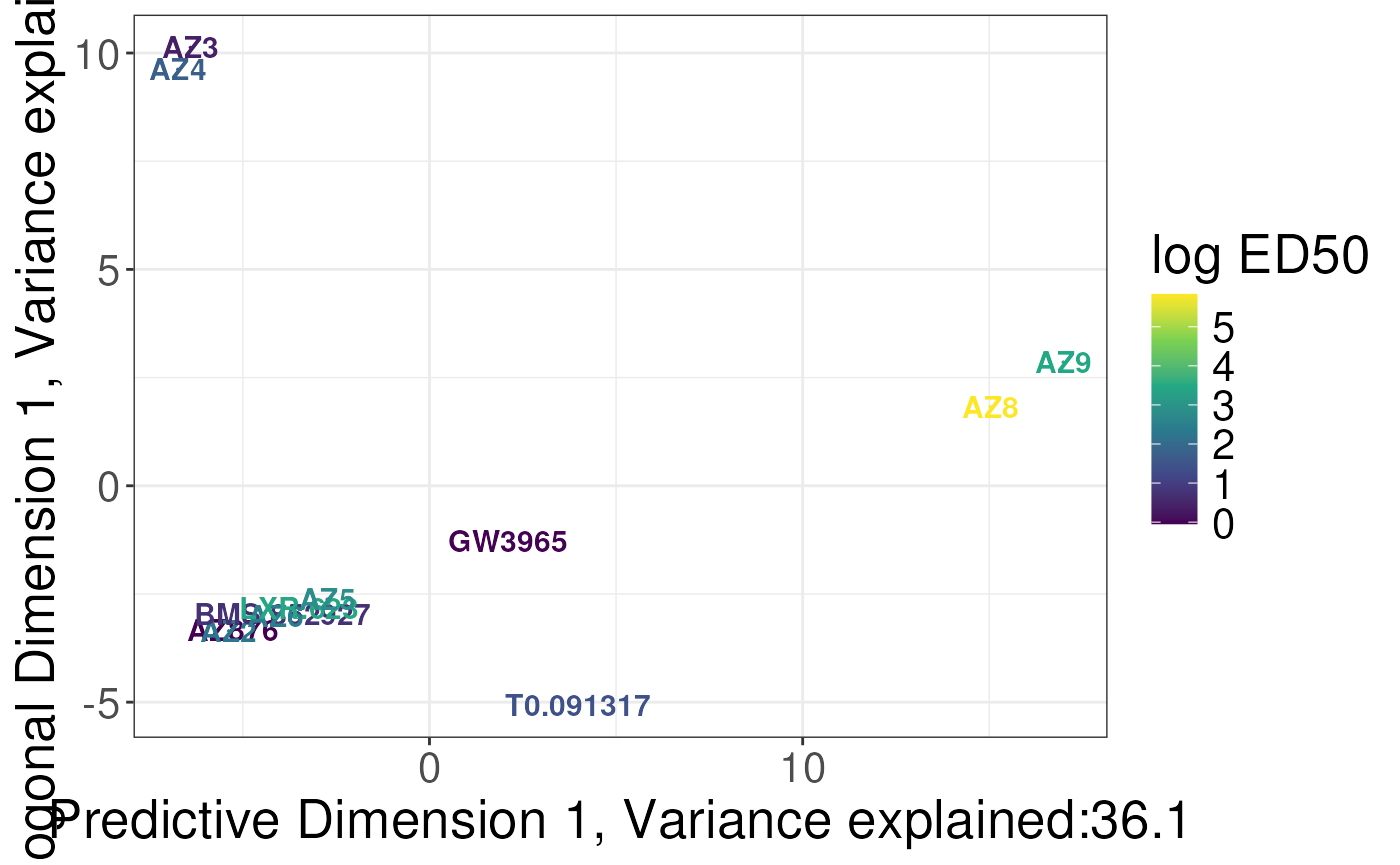
plotLoadingSCSA(states.plsda = scsa3,
                labels = labels,
                whichLoading = "predictive",
                whichlabel = "ED50")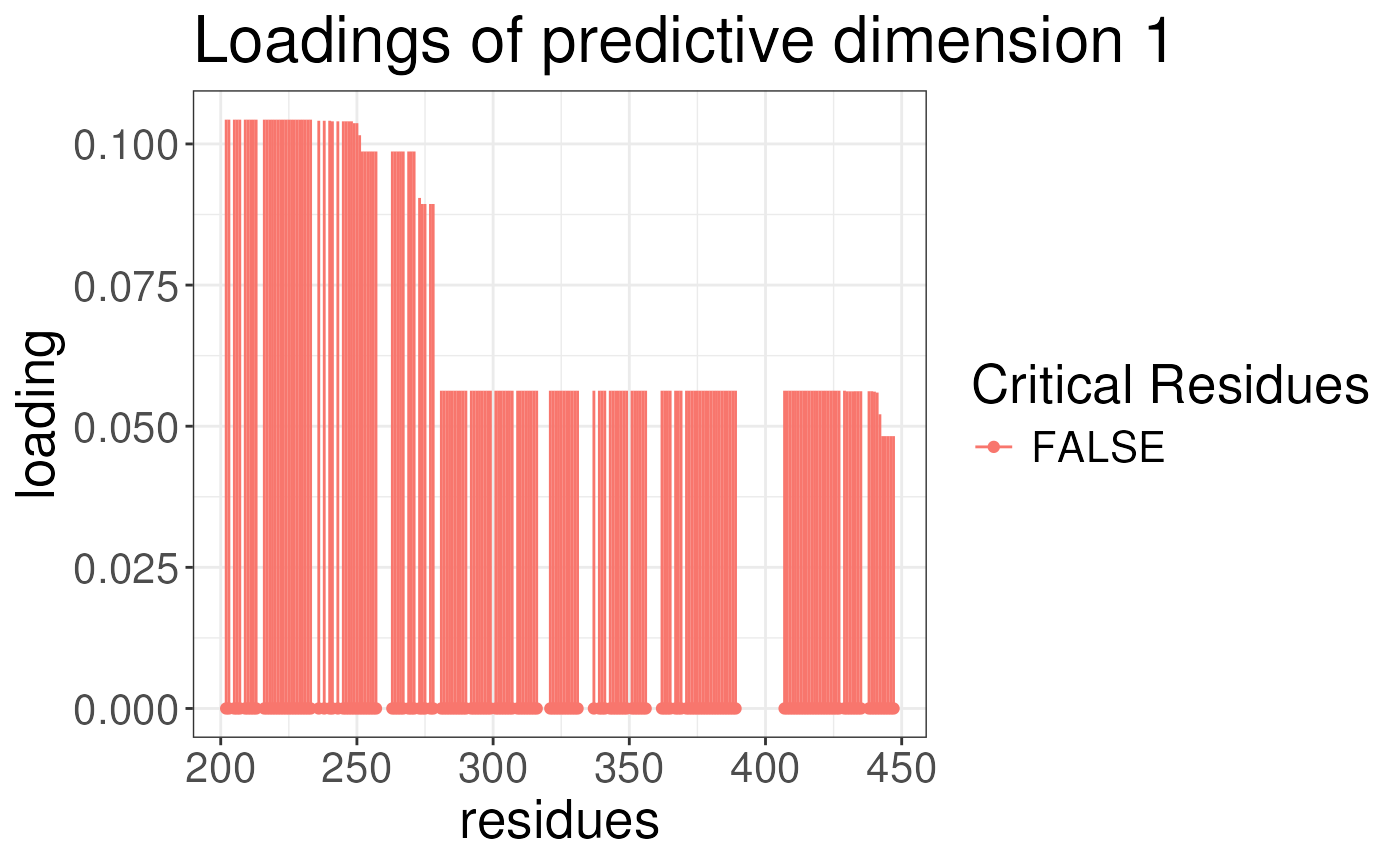
plotLoadingSCSA(states.plsda = scsa3,
                labels = labels,
                whichLoading = "orthogonal",
                whichlabel = "ED50")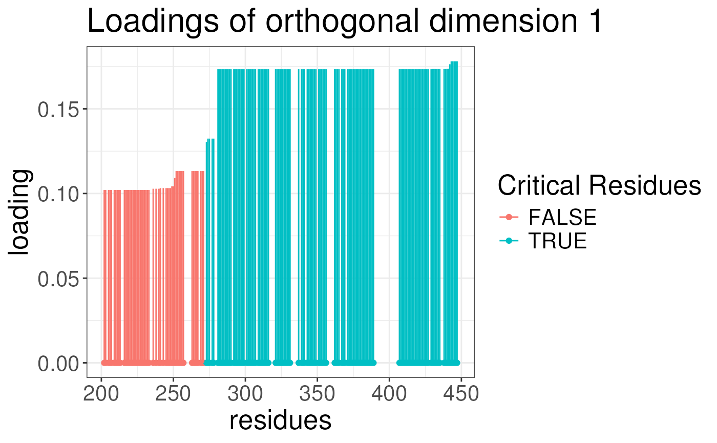
Advanced analysis
Until now we havent used the uncertainty in the analysis. We can use
the uncertainty in the analysis to generate the conformational
signature. We sample from the distribution of the parameters to generate
the conformational signature. We will use the
sampleTREuncertainty function. This function will take the
outputs of the analysis and sample from the distribution of the
parameters to quantify the uncertainty in the conformational signature.
The important argument below is the num_montecarlo which is
the number of samples to take from the distribution. We will set this to
5000. The whichSamples argument is the samples to use from
the orginal analysis. We will use the first 50 samples - note that since
the results have been processed the samples are actually the first 50
samples of the processed results.
We will not run the code here but pre-load the results from the package.
TRE_dist <- sampleTREuncertainty(HdxData = LXRalpha_processed,
                     RexParamsList = rex_lxr,
                     quantity = "TRE",
                     states = states,
                     whichChain = 1,
                     whichSamples = seq.int(1, 50),
                     whichTimepoint = 600,
                     num_montecarlo = 5000)
We will now load the results from the package. The results are stored
in the TRE_dist object.
data("TRE_dist")To plot the results we will use the
plotTREuncertaintyLoadings function. This function will
take the output of the sampleTREuncertainty function and
plot the results. We also need to pass the pca_states
object from the unsupervised analysis. We will plot the results. This
analysis reports the distribution of the loadings.
gg <- plotTREuncertaintyLoadings(df_all = TRE_dist,
pca_states = ucsa$pca_states,
states = states)
gg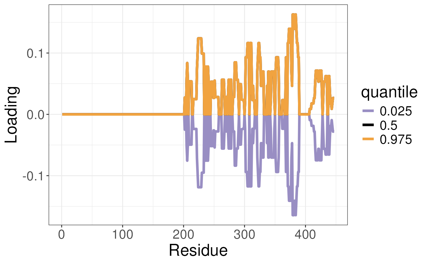 To visualise the results we can use the
 plotTREuncertainty
function. This function will take the output of the
sampleTREuncertainty function and plot the results. We also
need to pass the pca_states object from the unsupervised
analysis. This plots the unsupervised analysis with the uncertainty as
contours in the pca coordinates.
Again the results suffer because of the lack of iterations in the analysis.
plotTREuncertainty(df_all = TRE_dist,
                   pca_states = ucsa$pca_states,
                   states = states)
## Warning: Duplicated aesthetics after name standardisation:
## contour## Warning: `stat_contour()`: Zero contours were generated## Warning in min(x): no non-missing arguments to min; returning Inf## Warning in max(x): no non-missing arguments to max; returning -Inf## Warning: `stat_contour()`: Zero contours were generated## Warning in min(x): no non-missing arguments to min; returning Inf## Warning in max(x): no non-missing arguments to max; returning -Inf## Warning: `stat_contour()`: Zero contours were generated## Warning in min(x): no non-missing arguments to min; returning Inf## Warning in max(x): no non-missing arguments to max; returning -Inf## Warning: `stat_contour()`: Zero contours were generated## Warning in min(x): no non-missing arguments to min; returning Inf## Warning in max(x): no non-missing arguments to max; returning -Inf## Warning: `stat_contour()`: Zero contours were generated## Warning in min(x): no non-missing arguments to min; returning Inf## Warning in max(x): no non-missing arguments to max; returning -Inf## Warning: `stat_contour()`: Zero contours were generated## Warning in min(x): no non-missing arguments to min; returning Inf## Warning in max(x): no non-missing arguments to max; returning -Inf## Warning: `stat_contour()`: Zero contours were generated## Warning in min(x): no non-missing arguments to min; returning Inf## Warning in max(x): no non-missing arguments to max; returning -Inf## Warning: `stat_contour()`: Zero contours were generated## Warning in min(x): no non-missing arguments to min; returning Inf## Warning in max(x): no non-missing arguments to max; returning -Inf## Warning: `stat_contour()`: Zero contours were generated## Warning in min(x): no non-missing arguments to min; returning Inf## Warning in max(x): no non-missing arguments to max; returning -Inf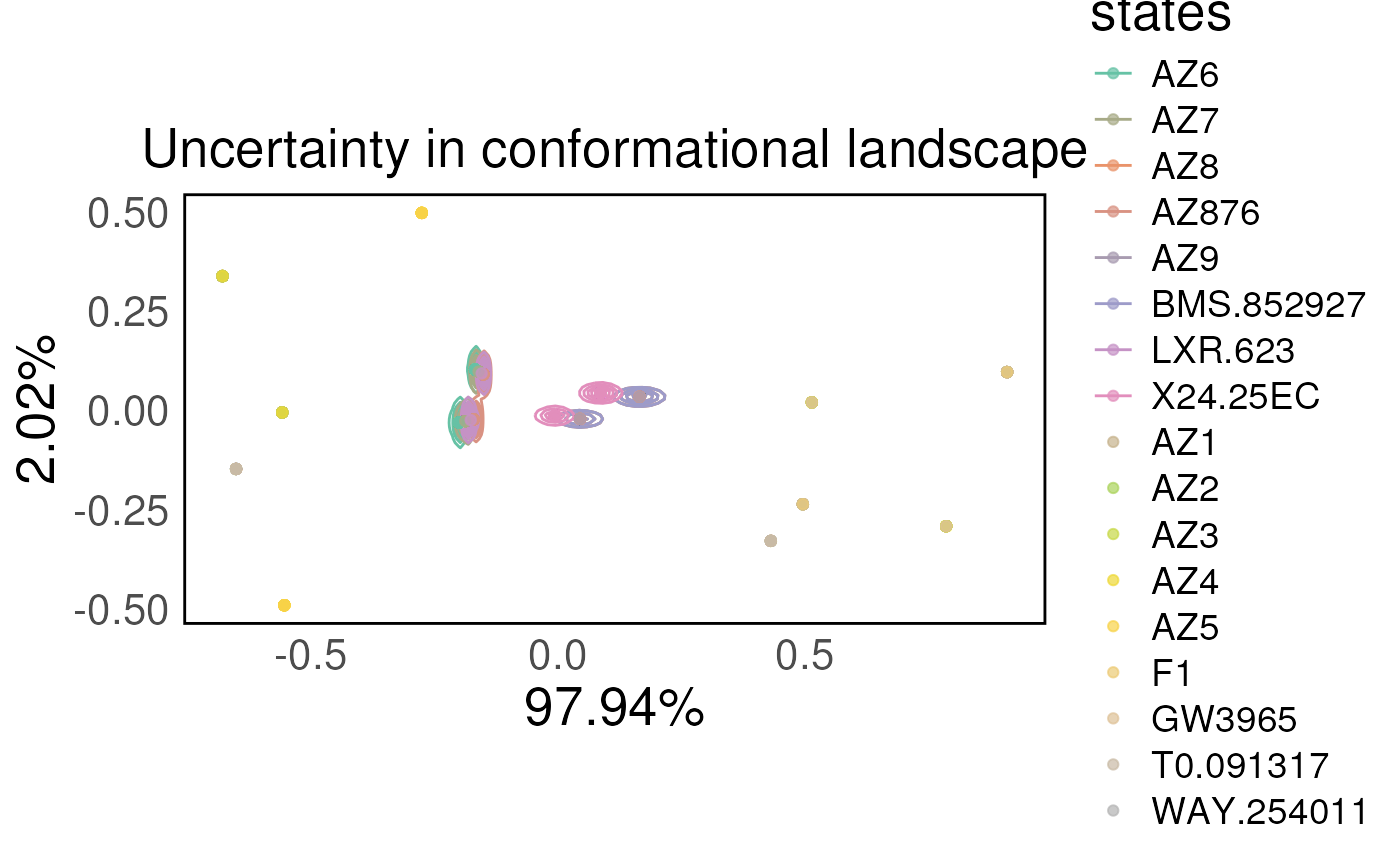
You may be interested in plotting the results of the analys on the structure. This is the same set-up as before you simply need to make sure that you align the residue numbers correctly
# Using the predictive component of the supervised analysis as an example
library(NGLVieweR)
library(dplyr)
##
## Attaching package: 'dplyr'## The following objects are masked from 'package:S4Vectors':
##
## first, intersect, rename, setdiff, setequal, union## The following objects are masked from 'package:BiocGenerics':
##
## combine, intersect, setdiff, union## The following objects are masked from 'package:stats':
##
## filter, lag## The following objects are masked from 'package:base':
##
## intersect, setdiff, setequal, union
v <- matrix(t(scsa@loadingMN), nrow = 1)

# set colnames carefully to residue number by first remove the x from the rownames
# and then coverting to numeric
colnames(v) <- as.numeric(gsub("x", "", rownames(scsa@loadingMN)))
pdb_filepath <- system.file("extdata", "2acl.pdb", mustWork = TRUE,
                            package = "RexMS")

mycolor_parameters <- hdx_to_pdb_colours(dataset = v,
                                         pdb = pdb_filepath,
                                         cmap_name = "CSA", scale_limits = c(-0.2,0))
## 2024-06-02 13:30:28.850248 [INFO] Your HDX input dataset has 184 entries
## 2024-06-02 13:30:28.850552 [INFO] And excluding NA data you only have 184 entries
## 2024-06-02 13:30:28.850642 [INFO] However, your input PDB has only 1827 residues in total
## 2024-06-02 13:30:28.851295 [INFO] Your scale limits are -0.2
## 2024-06-02 13:30:28.851295 [INFO] Your scale limits are 0
## 2024-06-02 13:30:28.851391 [INFO] Your values will be coloured using custom format
graphics <- NGLVieweR(pdb_filepath) %>%
  stageParameters(backgroundColor = "white", zoomSpeed = 1) %>%
  addRepresentation("ribbon") %>%   setQuality("high") %>%
  addRepresentation("ribbon", param = list(color=mycolor_parameters,
                                           backgroundColor="white"))

graphics
To extract the information from the uncertainty quantification analysis:
# Using the lower quantile as an example
loadingquants <- gg$data

v <- matrix(as.numeric(loadingquants[loadingquants$level == 0.025,
                                     "quantile", drop = FALSE][[1]]), nrow = 1)
colnames(v) <- seq.int(ncol(v))
pdb_filepath <- system.file("extdata", "2acl.pdb", mustWork = TRUE,
                            package = "RexMS")


mycolor_parameters <- hdx_to_pdb_colours(dataset = v,
                                         pdb = pdb_filepath,
                                         cmap_name = "CSA")
## 2024-06-02 13:30:29.216062 [INFO] Your HDX input dataset has 447 entries
## 2024-06-02 13:30:29.216193 [INFO] And excluding NA data you only have 447 entries
## 2024-06-02 13:30:29.216285 [INFO] However, your input PDB has only 1827 residues in total
## 2024-06-02 13:30:29.216867 [INFO] Your scale limits are -0.16
## 2024-06-02 13:30:29.216867 [INFO] Your scale limits are 0
## 2024-06-02 13:30:29.21696 [INFO] Your values will be coloured using custom format
graphics <- NGLVieweR(pdb_filepath) %>%
  stageParameters(backgroundColor = "white", zoomSpeed = 1) %>%
  addRepresentation("ribbon") %>%   setQuality("high") %>%
  addRepresentation("ribbon", param = list(color=mycolor_parameters,
                                           backgroundColor="white"))

graphics
R session information.
## ─ Session info ───────────────────────────────────────────────────────────────────────────────────────────────────────
##  setting  value
##  version  R version 4.3.3 (2024-02-29)
##  os       Ubuntu 22.04.4 LTS
##  system   x86_64, linux-gnu
##  ui       X11
##  language en
##  collate  en_US.UTF-8
##  ctype    en_US.UTF-8
##  tz       UTC
##  date     2024-06-02
##  pandoc   3.1.1 @ /usr/local/bin/ (via rmarkdown)
##
## ─ Packages ───────────────────────────────────────────────────────────────────────────────────────────────────────────
##  package              * version    date (UTC) lib source
##  abind                  1.4-5      2016-07-21 [1] RSPM (R 4.3.0)
##  bio3d                  2.4-4      2022-10-26 [1] RSPM (R 4.3.0)
##  Biobase                2.62.0     2023-10-24 [1] Bioconductor
##  BiocGenerics         * 0.48.1     2023-11-01 [1] Bioconductor
##  BiocManager            1.30.22    2023-08-08 [1] RSPM (R 4.3.0)
##  BiocParallel           1.36.0     2023-10-24 [1] Bioconductor
##  BiocStyle            * 2.30.0     2023-10-24 [1] Bioconductor
##  bitops                 1.0-7      2021-04-24 [1] RSPM (R 4.3.0)
##  bookdown               0.39       2024-04-15 [1] RSPM (R 4.3.0)
##  bslib                  0.7.0      2024-03-29 [2] RSPM (R 4.3.0)
##  cachem                 1.0.8      2023-05-01 [2] RSPM (R 4.3.0)
##  calibrate              1.7.7      2020-06-19 [1] RSPM (R 4.3.0)
##  cli                    3.6.2      2023-12-11 [2] RSPM (R 4.3.0)
##  cluster                2.1.6      2023-12-01 [3] CRAN (R 4.3.3)
##  coda                   0.19-4.1   2024-01-31 [1] RSPM (R 4.3.0)
##  codetools              0.2-20     2024-03-31 [3] RSPM (R 4.3.0)
##  colorspace             2.1-0      2023-01-23 [1] RSPM (R 4.3.0)
##  comprehenr             0.6.10     2021-01-31 [1] RSPM (R 4.3.0)
##  crayon                 1.5.2      2022-09-29 [2] RSPM (R 4.3.0)
##  DBI                    1.2.2      2024-02-16 [1] RSPM (R 4.3.0)
##  dbplyr                 2.5.0      2024-03-19 [1] RSPM (R 4.3.0)
##  DelayedArray           0.28.0     2023-10-24 [1] Bioconductor
##  desc                   1.4.3      2023-12-10 [2] RSPM (R 4.3.0)
##  digest                 0.6.35     2024-03-11 [2] RSPM (R 4.3.0)
##  dplyr                * 1.1.4      2023-11-17 [1] RSPM (R 4.3.0)
##  evaluate               0.23       2023-11-01 [2] RSPM (R 4.3.0)
##  fansi                  1.0.6      2023-12-08 [2] RSPM (R 4.3.0)
##  farver                 2.1.1      2022-07-06 [1] RSPM (R 4.3.0)
##  fastmap                1.1.1      2023-02-24 [2] RSPM (R 4.3.0)
##  fs                     1.6.3      2023-07-20 [2] RSPM (R 4.3.0)
##  generics               0.1.3      2022-07-05 [1] RSPM (R 4.3.0)
##  genlasso               1.6.1      2022-08-22 [1] RSPM (R 4.3.0)
##  GenomeInfoDb           1.38.8     2024-03-15 [1] Bioconductor 3.18 (R 4.3.2)
##  GenomeInfoDbData       1.2.11     2024-04-06 [1] Bioconductor
##  GenomicRanges          1.54.1     2023-10-29 [1] Bioconductor
##  ggfortify            * 0.4.17     2024-04-17 [1] RSPM (R 4.3.0)
##  ggplot2              * 3.5.0      2024-02-23 [1] RSPM (R 4.3.0)
##  glue                   1.7.0      2024-01-09 [2] RSPM (R 4.3.0)
##  gridExtra              2.3        2017-09-09 [1] RSPM (R 4.3.0)
##  gtable                 0.3.5      2024-04-22 [1] RSPM (R 4.3.0)
##  highr                  0.10       2022-12-22 [2] RSPM (R 4.3.0)
##  htmltools              0.5.8.1    2024-04-04 [2] RSPM (R 4.3.0)
##  htmlwidgets            1.6.4      2023-12-06 [2] RSPM (R 4.3.0)
##  httpuv                 1.6.15     2024-03-26 [2] RSPM (R 4.3.0)
##  igraph                 2.0.3      2024-03-13 [1] RSPM (R 4.3.0)
##  IRanges                2.36.0     2023-10-24 [1] Bioconductor
##  isoband                0.2.7      2022-12-20 [1] RSPM (R 4.3.0)
##  jquerylib              0.1.4      2021-04-26 [2] RSPM (R 4.3.0)
##  jsonlite               1.8.8      2023-12-04 [2] RSPM (R 4.3.0)
##  knitr                  1.46       2024-04-06 [2] RSPM (R 4.3.0)
##  labeling               0.4.3      2023-08-29 [1] RSPM (R 4.3.0)
##  LaplacesDemon          16.1.6     2021-07-09 [1] RSPM (R 4.3.0)
##  later                  1.3.2      2023-12-06 [2] RSPM (R 4.3.0)
##  lattice                0.22-6     2024-03-20 [3] RSPM (R 4.3.0)
##  lifecycle              1.0.4      2023-11-07 [2] RSPM (R 4.3.0)
##  limma                  3.58.1     2023-10-31 [1] Bioconductor
##  magrittr               2.0.3      2022-03-30 [2] RSPM (R 4.3.0)
##  MASS                   7.3-60.0.1 2024-01-13 [3] CRAN (R 4.3.3)
##  Matrix                 1.6-5      2024-01-11 [3] CRAN (R 4.3.3)
##  MatrixGenerics         1.14.0     2023-10-24 [1] Bioconductor
##  matrixStats            1.3.0      2024-04-11 [1] RSPM (R 4.3.0)
##  memoise                2.0.1      2021-11-26 [2] RSPM (R 4.3.0)
##  mgcv                   1.9-1      2023-12-21 [3] CRAN (R 4.3.3)
##  mime                   0.12       2021-09-28 [2] RSPM (R 4.3.0)
##  minpack.lm             1.2-4      2023-09-11 [1] RSPM (R 4.3.0)
##  MultiAssayExperiment   1.28.0     2023-10-24 [1] Bioconductor
##  MultiDataSet           1.30.0     2023-10-24 [1] Bioconductor
##  munsell                0.5.1      2024-04-01 [1] RSPM (R 4.3.0)
##  NGLVieweR            * 1.3.1      2021-06-01 [1] RSPM (R 4.3.0)
##  nlme                   3.1-164    2023-11-27 [3] CRAN (R 4.3.3)
##  permute                0.9-7      2022-01-27 [1] RSPM (R 4.3.0)
##  pheatmap               1.0.12     2019-01-04 [1] RSPM (R 4.3.0)
##  pillar                 1.9.0      2023-03-22 [2] RSPM (R 4.3.0)
##  pkgconfig              2.0.3      2019-09-22 [2] RSPM (R 4.3.0)
##  pkgdown                2.0.9      2024-04-18 [2] RSPM (R 4.3.0)
##  plyr                   1.8.9      2023-10-02 [1] RSPM (R 4.3.0)
##  promises               1.3.0      2024-04-05 [2] RSPM (R 4.3.0)
##  purrr                  1.0.2      2023-08-10 [2] RSPM (R 4.3.0)
##  qqman                  0.1.9      2023-08-23 [1] RSPM (R 4.3.0)
##  R6                     2.5.1      2021-08-19 [2] RSPM (R 4.3.0)
##  ragg                   1.3.0      2024-03-13 [2] RSPM (R 4.3.0)
##  RColorBrewer           1.1-3      2022-04-03 [1] RSPM (R 4.3.0)
##  Rcpp                   1.0.12     2024-01-09 [2] RSPM (R 4.3.0)
##  RCurl                  1.98-1.14  2024-01-09 [1] RSPM (R 4.3.0)
##  RexMS                * 0.99.7     2024-06-02 [1] Bioconductor
##  rlang                  1.1.3      2024-01-10 [2] RSPM (R 4.3.0)
##  rlog                   0.1.0      2021-02-24 [1] RSPM (R 4.3.0)
##  rmarkdown              2.26       2024-03-05 [2] RSPM (R 4.3.0)
##  ropls                  1.34.0     2023-10-24 [1] Bioconductor
##  S4Arrays               1.2.1      2024-03-04 [1] Bioconductor 3.18 (R 4.3.2)
##  S4Vectors            * 0.40.2     2023-11-23 [1] Bioconductor 3.18 (R 4.3.2)
##  sass                   0.4.9      2024-03-15 [2] RSPM (R 4.3.0)
##  scales                 1.3.0      2023-11-28 [1] RSPM (R 4.3.0)
##  sessioninfo          * 1.2.2      2021-12-06 [2] RSPM (R 4.3.0)
##  shiny                  1.8.1.1    2024-04-02 [2] RSPM (R 4.3.0)
##  SparseArray            1.2.4      2024-02-11 [1] Bioconductor 3.18 (R 4.3.2)
##  statmod                1.5.0      2023-01-06 [1] RSPM (R 4.3.0)
##  stringi                1.8.3      2023-12-11 [2] RSPM (R 4.3.0)
##  stringr                1.5.1      2023-11-14 [2] RSPM (R 4.3.0)
##  SummarizedExperiment   1.32.0     2023-10-24 [1] Bioconductor
##  systemfonts            1.0.6      2024-03-07 [2] RSPM (R 4.3.0)
##  textshaping            0.3.7      2023-10-09 [2] RSPM (R 4.3.0)
##  tibble                 3.2.1      2023-03-20 [2] RSPM (R 4.3.0)
##  tidyr                  1.3.1      2024-01-24 [1] RSPM (R 4.3.0)
##  tidyselect             1.2.1      2024-03-11 [1] RSPM (R 4.3.0)
##  utf8                   1.2.4      2023-10-22 [2] RSPM (R 4.3.0)
##  vctrs                  0.6.5      2023-12-01 [2] RSPM (R 4.3.0)
##  vegan                  2.6-4      2022-10-11 [1] RSPM (R 4.3.0)
##  viridisLite            0.4.2      2023-05-02 [1] RSPM (R 4.3.0)
##  withr                  3.0.0      2024-01-16 [2] RSPM (R 4.3.0)
##  xfun                   0.43       2024-03-25 [2] RSPM (R 4.3.0)
##  xtable                 1.8-4      2019-04-21 [2] RSPM (R 4.3.0)
##  XVector                0.42.0     2023-10-24 [1] Bioconductor
##  yaml                   2.3.8      2023-12-11 [2] RSPM (R 4.3.0)
##  zlibbioc               1.48.2     2024-03-13 [1] Bioconductor 3.18 (R 4.3.2)
##
##  [1] /__w/_temp/Library
##  [2] /usr/local/lib/R/site-library
##  [3] /usr/local/lib/R/library
##
## ──────────────────────────────────────────────────────────────────────────────────────────────────────────────────────